I wish to us ggplot2 in RStudio to make a diagram which displays the acceptance regions of my null hypothesis given my data. I know that I must use the function ggplot() although I don't know what to enter in as the parameters and how to make it specific for what I want. Also I am not sure what kind of data I should be entering in since I have different types of values I found, if anyone can inform me some more on how to perform the tailed statistical tests this way I would appreciate a lot.
Here is an example where the null distribution is a t-distribution. The blue vertical bars represent the significance thresholds at the 0.05 significance level.
library(ggplot2)
set.seed(123)

## Generate 10 random values from a normal distribution and compute test statistic for the mean
sample=rnorm(n=10,mean=1,sd=1)
sample_statistic=mean(sample)/(sd(sample)/sqrt(length(sample)))

## Compute upper and lower significance thresholds
lower=qt(p=0.05,df=9,lower.tail=TRUE)
upper=qt(p=0.05,df=9,lower.tail=FALSE)

## Create data for the null distribution, a t-distribution with 10-1=9 d.f.
plot_data=data.frame(x=seq(-5,5,0.001),y=sapply(seq(-5,5,0.001),function(x){dt(x=x,df=9)}))

## Create the plot with blue vertical bars for significance thresholds and a red vertical bar for the observed sample
(plot=ggplot(data=plot_data,aes(x=x,y=y))+
  geom_line()+
  geom_vline(xintercept=c(lower,upper),color="blue")+geom_vline(xintercept=sample_statistic,color="red"))
In the future, if you don't want to use a graph, you can also compute a p-value for a two-sided test:
2*pt(sample_statistic,df=9,lower.tail=FALSE)
You can change the t-distribution to the distribution that fits your purpose. For example, dt, "t density", could be replaced by the normal density, dnorm, and the quantile function qt by qnorm. In that case you won't need the degrees of freedom argument.
This is a great resource to get you started, specifically Chapter 3 on data visualization. It will walk you through the basics on ggplot and help you make your first visualization.
Hope this helps!
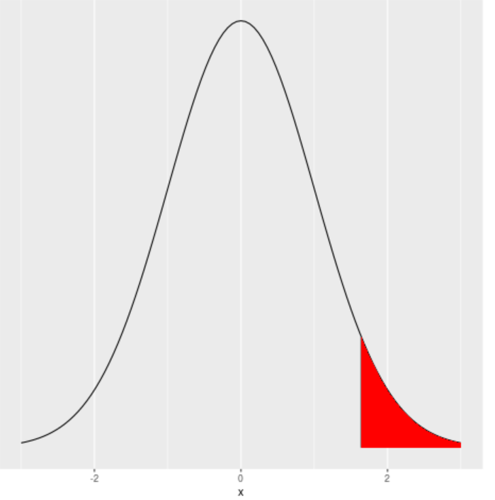
This is both a statistical question and an R question. The statistical question would take a chapter to answer in general. Let's simplify it to one small case. Suppose you have a normal curve with mean 0 and SD 1, and you wish to reject the null hypothesis when the probability is in the 5% right tail. That critical z value is qnorm(.95) which is 1.644854. The following code graphs a normal curve and shades the critical region.
library(ggplot2)
z <- qnorm(.95)
ggplot(data = data.frame(x = c(-3, 3)), aes(x)) +
stat_function(fun = dnorm, n = 101, args = list(mean = 0, sd = 1)) + ylab("") +
scale_y_continuous(breaks = NULL) +
geom_segment(x = z, y = 0, xend = z, yend = dnorm(z, mean = 0, sd = 1)) +
stat_function(fun = dnorm, geom = "area", fill = "red", xlim = c(z, 3))
2 Likes
This topic was automatically closed 21 days after the last reply. New replies are no longer allowed.
If you have a query related to it or one of the replies, start a new topic and refer back with a link.