Spearman correlation

[Galal]

Hello everyone,

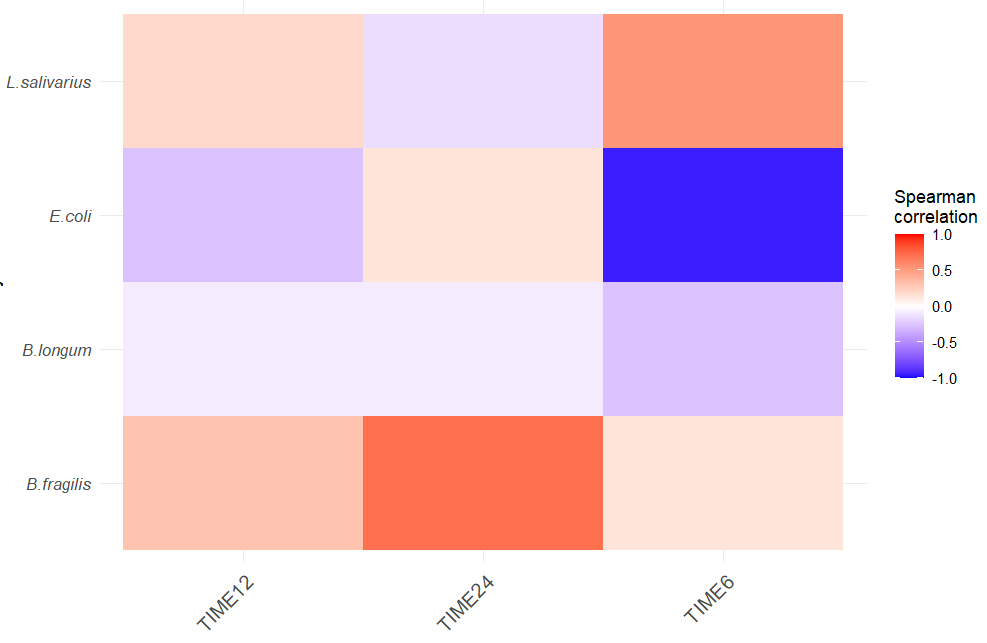
I'm using ggplot2 to create a correlation heatmap, I'm trying to add the p value as stars (***) inside the figure, this is the script that was used:
library(corrr)
library(dplyr)
library(ggplot2)
my_data<- read.delim("input_data.txt", header = T)
my_data
X E.coli L.salivarius B.fragilis B.longum TIME6 TIME12
1 R1 0.008238399 0.037155326 0.005557831 0.023688994 1.776333 4.25300
2 R2 0.001297156 0.090566197 0.007841161 0.012975925 8.140000 18.24925
3 R3 0.002386935 0.062769327 0.024554017 0.015576090 5.125875 14.66462
4 R4 0.002016223 0.006694006 0.008878337 0.007006086 7.150500 13.97425
5 R5 0.003888820 0.001150177 0.008036232 0.003939090 3.910125 14.36300
6 R6 0.015246245 0.000144155 0.012469594 0.008493679 3.214625 16.73150
TIME24
1 16.39300
2 25.48738
3 25.98112
4 16.58438
5 18.49750
6 33.40962
hp <-
my_data %>%
correlate(method = "spearman") %>%
stretch()

hp %>%
ggplot(aes(x, y, fill = r)) +
geom_tile()

x and y axes for the heatmaps

hp_filtered <-
hp %>%
filter(
y %in% c("E.coli", "L.salivarius", "B.fragilis", "B.longum"),
x %in% c("TIME6", "TIME12", "TIME24"))

hp_filtered %>%
ggplot(aes(x, y, fill = r)) +
geom_tile() + scale_fill_gradient2(low = "blue", high = "red", mid = "white",
midpoint = 0, limit = c(-1,1), space = "Lab",
name="Spearman\ncorrelation") +
theme_minimal() +
theme(axis.text.x = element_text(angle = 45, vjust = 1,
size = 12, hjust = 1)) +
theme(axis.text.y = element_text(face ="italic","bold",
size = 10,))
the output

I appreciate your help in advance
thank you

[DavoWW]

Hi @Galal
I couldn't see a simple way to get the P values for the correlations via the {corrr} package but the {Hmisc} does provide the required output:

suppressPackageStartupMessages(library(tidyverse))
library(Hmisc)
#> 
#> Attaching package: 'Hmisc'
#> The following objects are masked from 'package:dplyr':
#> 
#>     src, summarize
#> The following objects are masked from 'package:base':
#> 
#>     format.pval, units

# Change one column name in TIME06 to get correct ordering
my_data<- read.delim(header = TRUE, sep=" ", text="
X E.coli L.salivarius B.fragilis B.longum TIME06 TIME12 TIME24
R1 0.008238399 0.037155326 0.005557831 0.023688994 1.776333 4.25300 16.39300
R2 0.001297156 0.090566197 0.007841161 0.012975925 8.140000 18.24925 25.48738
R3 0.002386935 0.062769327 0.024554017 0.015576090 5.125875 14.66462 25.98112
R4 0.002016223 0.006694006 0.008878337 0.007006086 7.150500 13.97425 16.58438
R5 0.003888820 0.001150177 0.008036232 0.003939090 3.910125 14.36300 18.49750
R6 0.015246245 0.000144155 0.012469594 0.008493679 3.214625 16.73150 33.40962
")

out <- rcorr(as.matrix(my_data[,2:8]), type = c("spearman"))

out$r
#>                   E.coli L.salivarius  B.fragilis    B.longum     TIME06
#> E.coli        1.00000000   -0.7142857  0.08571429  0.08571429 -0.9428571
#> L.salivarius -0.71428571    1.0000000 -0.25714286  0.60000000  0.5428571
#> B.fragilis    0.08571429   -0.2571429  1.00000000 -0.20000000  0.1428571
#> B.longum      0.08571429    0.6000000 -0.20000000  1.00000000 -0.2571429
#> TIME06       -0.94285714    0.5428571  0.14285714 -0.25714286  1.0000000
#> TIME12       -0.25714286    0.2000000  0.31428571 -0.08571429  0.4857143
#> TIME24        0.14285714   -0.1428571  0.71428571 -0.08571429  0.1428571
#>                   TIME12      TIME24
#> E.coli       -0.25714286  0.14285714
#> L.salivarius  0.20000000 -0.14285714
#> B.fragilis    0.31428571  0.71428571
#> B.longum     -0.08571429 -0.08571429
#> TIME06        0.48571429  0.14285714
#> TIME12        1.00000000  0.82857143
#> TIME24        0.82857143  1.00000000
out$P
#>                   E.coli L.salivarius B.fragilis  B.longum      TIME06
#> E.coli                NA    0.1107872  0.8717434 0.8717434 0.004804665
#> L.salivarius 0.110787172           NA  0.6227872 0.2080000 0.265702624
#> B.fragilis   0.871743440    0.6227872         NA 0.7040000 0.787172012
#> B.longum     0.871743440    0.2080000  0.7040000        NA 0.622787172
#> TIME06       0.004804665    0.2657026  0.7871720 0.6227872          NA
#> TIME12       0.622787172    0.7040000  0.5440933 0.8717434 0.328723032
#> TIME24       0.787172012    0.7871720  0.1107872 0.8717434 0.787172012
#>                  TIME12     TIME24
#> E.coli       0.62278717 0.78717201
#> L.salivarius 0.70400000 0.78717201
#> B.fragilis   0.54409329 0.11078717
#> B.longum     0.87174344 0.87174344
#> TIME06       0.32872303 0.78717201
#> TIME12               NA 0.04156268
#> TIME24       0.04156268         NA

# See: http://sthda.com/english/wiki/correlation-matrix-a-quick-start-guide-to-analyze-format-and-visualize-a-correlation-matrix-using-r-software
# ++++++++++++++++++++++++++++
# flattenCorrMatrix
# ++++++++++++++++++++++++++++
# cormat : matrix of the correlation coefficients
# pmat : matrix of the correlation p-values
flattenCorrMatrix <- function(cormat, pmat) {
  ut <- upper.tri(cormat)
  data.frame(
    row = rownames(cormat)[row(cormat)[ut]],
    column = rownames(cormat)[col(cormat)[ut]],
    cor  =(cormat)[ut],
    p = pmat[ut]
    )
}

hp <- flattenCorrMatrix(out$r, out$P)

hp_filtered <- hp %>%
                filter(row %in% c("E.coli", "L.salivarius", "B.fragilis", "B.longum"),
                       column %in% c("TIME06", "TIME12", "TIME24"))

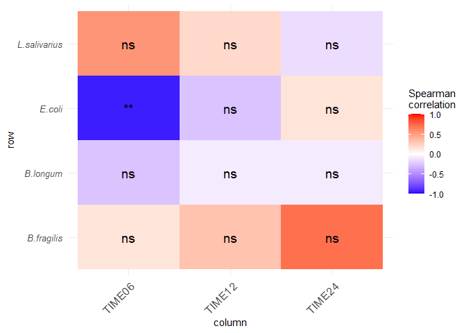
hp_filtered %>% 
  mutate(sig_text = case_when(
                      p >= 0.05 ~ "ns",
                      0.05 > p & p > 0.01 ~ "*",
                      0.01 >= p & p > 0.001 ~ "**",
                      p <=0.001 ~ "***",
                      .default = "error")) -> hp_filtered

hp_filtered %>%
  ggplot(aes(column, row, fill = cor)) +
  geom_tile() + 
  scale_fill_gradient2(low = "blue", high = "red", mid = "white",
                       midpoint = 0, limit = c(-1,1), space = "Lab",
                       name="Spearman\ncorrelation") +
  geom_text(label=hp_filtered$sig_text, size=5) +
  theme_minimal() +
  theme(axis.text.x = element_text(angle = 45, vjust = 1, size = 12, hjust = 1)) +
  theme(axis.text.y = element_text(face ="italic", size = 10))

^{Created on 2023-05-28 with reprex v2.0.2}

[Galal]

Hi @DavoWW
I'm so grateful,
Thanks for your work on it