Adding Percentages to Top of Histogram

Dan0o0o · September 30, 2022, 4:26pm

Been working on this project and nearing completion... my code is below and associated viz.

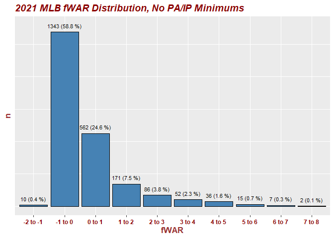
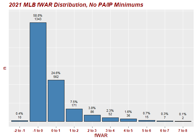
I want to add a percentage to the top of each histogram bar/column WHILE MAINTAINING counts in the X axis. The counts are there but how do I add percentages to each inside the bar or above the counts above the bar (indifferent on the cosmetics here)?

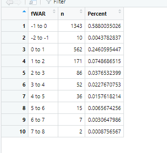
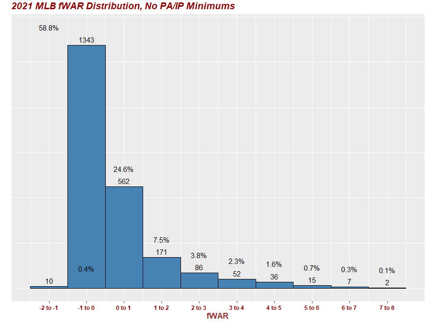
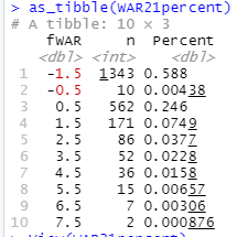
In my DataFrames for this first ggplot (WAR21percent which is pictured at the bottom of this post) I have a Percent column with the numbers I want (would like to get it down to one decimal point, but that's another story and issue) from this dataframe to get onto the viz.

Where can I add this in? I used stat_bin to get the counts on the x axis. How can I add percents? Open to and appreciate all recs!

library(dplyr)
library(base)
library(dplyr)
library(tidyverse)
WAR <- read.csv("WAR.csv")
View(WAR)
## Only Pitchers displayed in a DF
pitchers <- filter(WAR, Type == "Pitcher")
View(pitchers)
##2020 pitchers only
pitchers20 <- filter(pitchers, year == 2020)
View(pitchers20)
##2021 pitchers only
pitchers21 <- filter(pitchers, year == 2021)
View(pitchers21)
##Only Hitters displayed in a DF
hitters <- filter(WAR, Type == "Hitter")
##2020 hitters only
hitters20 <- filter(hitters, year == 2020)
##2021 hitters only
hitters21 <- filter(hitters, year == 2021)
##2020 all WAR
WAR20 <- filter (WAR, year ==2020)
#2021 all WAR
WAR21 <- filter( WAR, year == 2021)

View(WAR21)

#Summary counts of the datasets
WAR21_labels = WAR21 %>% 
  count(WAR)

#Summary counts of the datasets 2020
WAR20_labels = WAR20 %>% 
  count(WAR)

pitchers21_labels = pitchers21 %>% 
  count(WAR)

pitchers20_labels = pitchers20 %>% 
  count(WAR)

hitters20_labels = hitters20 %>% 
  count(WAR)

hitters21_labels = hitters21 %>% 
  count(WAR)

View(WAR21_labels)

View(WAR20_labels)

View(pitchers21)

##Using case_when to create WAR bins and then counting up these bins using count function for 2021 ALL

WAR21_subset <- WAR21 %>%
  mutate(fWAR = case_when(WAR >= -2 & WAR <= -1 ~ "-2 to -1",
                          WAR >= -1 & WAR <= 0 ~ "-1 to 0",
                          WAR >= 0 & WAR <= 1 ~ "0 to 1",
                          WAR >= 1 & WAR <= 2 ~ "1 to 2",
                          WAR >= 2 & WAR <= 3 ~ "2 to 3",
                          WAR >= 3 & WAR <= 4 ~ "3 to 4",
                          WAR >= 4 & WAR <= 5 ~ "4 to 5",
                          WAR >= 5 & WAR <= 6 ~ "5 to 6",
                          WAR >= 6 & WAR <= 7 ~ "6 to 7",
                          WAR >= 7 & WAR <= 8 ~ "7 to 8",))


WAR21_labels =  WAR21_subset %>%
  count(fWAR)

##For 2020 ALL

WAR20_subset <- WAR20 %>%
  mutate(fWAR = case_when(WAR >= -2 & WAR <= -1 ~ "-2 to -1",
                          WAR >= -1 & WAR <= 0 ~ "-1 to 0",
                          WAR >= 0 & WAR <= 1 ~ "0 to 1",
                          WAR >= 1 & WAR <= 2 ~ "1 to 2",
                          WAR >= 2 & WAR <= 3 ~ "2 to 3",
                          WAR >= 3 & WAR <= 4 ~ "3 to 4",
                          WAR >= 4 & WAR <= 5 ~ "4 to 5",
                          WAR >= 5 & WAR <= 6 ~ "5 to 6",
                          WAR >= 6 & WAR <= 7 ~ "6 to 7",
                          WAR >= 7 & WAR <= 8 ~ "7 to 8",))


WAR20_labels =  WAR20_subset %>%
  count(fWAR)

##For 2021 pitchers

pitchers21_subset <- pitchers21 %>%
  mutate(fWAR = case_when(WAR >= -2 & WAR <= -1 ~ "-2 to -1",
                          WAR >= -1 & WAR <= 0 ~ "-1 to 0",
                          WAR >= 0 & WAR <= 1 ~ "0 to 1",
                          WAR >= 1 & WAR <= 2 ~ "1 to 2",
                          WAR >= 2 & WAR <= 3 ~ "2 to 3",
                          WAR >= 3 & WAR <= 4 ~ "3 to 4",
                          WAR >= 4 & WAR <= 5 ~ "4 to 5",
                          WAR >= 5 & WAR <= 6 ~ "5 to 6",
                          WAR >= 6 & WAR <= 7 ~ "6 to 7",
                          WAR >= 7 & WAR <= 8 ~ "7 to 8",))


pitchers21_labels =  pitchers21_subset %>%
  count(fWAR)

##For 2020 pitchers

pitchers20_subset <- pitchers20 %>%
  mutate(fWAR = case_when(WAR >= -2 & WAR <= -1 ~ "-2 to -1",
                          WAR >= -1 & WAR <= 0 ~ "-1 to 0",
                          WAR >= 0 & WAR <= 1 ~ "0 to 1",
                          WAR >= 1 & WAR <= 2 ~ "1 to 2",
                          WAR >= 2 & WAR <= 3 ~ "2 to 3",
                          WAR >= 3 & WAR <= 4 ~ "3 to 4",
                          WAR >= 4 & WAR <= 5 ~ "4 to 5",
                          WAR >= 5 & WAR <= 6 ~ "5 to 6",
                          WAR >= 6 & WAR <= 7 ~ "6 to 7",
                          WAR >= 7 & WAR <= 8 ~ "7 to 8",))


pitchers20_labels =  pitchers20_subset %>%
  count(fWAR)

##for 2020 hitters
hitters20_subset <- hitters20 %>%
  mutate(fWAR = case_when(WAR >= -2 & WAR <= -1 ~ "-2 to -1",
                          WAR >= -1 & WAR <= 0 ~ "-1 to 0",
                          WAR >= 0 & WAR <= 1 ~ "0 to 1",
                          WAR >= 1 & WAR <= 2 ~ "1 to 2",
                          WAR >= 2 & WAR <= 3 ~ "2 to 3",
                          WAR >= 3 & WAR <= 4 ~ "3 to 4",
                          WAR >= 4 & WAR <= 5 ~ "4 to 5",
                          WAR >= 5 & WAR <= 6 ~ "5 to 6",
                          WAR >= 6 & WAR <= 7 ~ "6 to 7",
                          WAR >= 7 & WAR <= 8 ~ "7 to 8",))


hitters20_labels =  hitters20_subset %>%
  count(fWAR)

##for 2021 hitters
hitters21_subset <- hitters21 %>%
  mutate(fWAR = case_when(WAR >= -2 & WAR <= -1 ~ "-2 to -1",
                          WAR >= -1 & WAR <= 0 ~ "-1 to 0",
                          WAR >= 0 & WAR <= 1 ~ "0 to 1",
                          WAR >= 1 & WAR <= 2 ~ "1 to 2",
                          WAR >= 2 & WAR <= 3 ~ "2 to 3",
                          WAR >= 3 & WAR <= 4 ~ "3 to 4",
                          WAR >= 4 & WAR <= 5 ~ "4 to 5",
                          WAR >= 5 & WAR <= 6 ~ "5 to 6",
                          WAR >= 6 & WAR <= 7 ~ "6 to 7",
                          WAR >= 7 & WAR <= 8 ~ "7 to 8",))


hitters21_labels =  hitters21_subset %>%
  count(fWAR)


View(pitchers21_labels)

View(WAR20_subset)

View(WAR21_subset)

View(WAR21_labels)

View(pitchers20_labels)

View(pitchers20)

as_tibble(hitters21)

View(hitters21)

as_tibble(hitters20)

View(WAR21)

library(scales)

##adding percent to the dataFrame. How do I add it above the histogram below???
WAR21percent <- WAR21_labels %>% 
  mutate(Percent = n/2284)

##adding percent to the 2020 dataFrame. How do I add it above the histogram below???
WAR20percent <- WAR20_labels %>% 
  mutate(Percent = n/1356)

pitchers21percent <- pitchers21_labels %>% 
  mutate(Percent = n/909)

pitchers20percent <- pitchers20_labels %>% 
  mutate(Percent = n/735)

hitters21percent <- hitters21_labels %>% 
  mutate(Percent = n/1375)

hitters20percent <- hitters20_labels %>% 
  mutate(Percent = n/621)

View(WAR20percent)  

View(WAR21percent)

View(pitchers21percent)

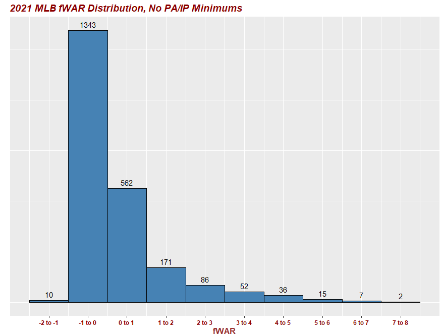
##histogram with WAR bins and totals above each bin 2021
ggplot(WAR21, aes(x=WAR))+
  geom_histogram(fill='steelblue', col='black', binwidth=1, center=0.5)+
  stat_bin(aes (y=..count.., label=..count..), geom="text", binwidth=1, center=0.5, vjust=-.5) +
  labs(title = "2021 MLB fWAR Distribution, No PA/IP Minimums")+
  scale_x_continuous(breaks = seq(-1.5, 7.5, by = 1.0),
                     # updating bin labels (same length as breaks)
                     labels = c('-2 to -1', '-1 to 0', '0 to 1', '1 to 2', '2 to 3', '3 to 4', '4 to 5', '5 to 6', '6 to 7', '7 to 8'))+
  ylab ("")+
  xlab("fWAR")+
  # updating to removes y-axis counts and ticks
  theme(axis.text.y = element_blank()) +
  theme(axis.ticks.y = element_blank()) +
  theme(axis.title.y = element_text(color="#993333", size=13, face="bold"))+
  theme(axis.title.x = element_text(color="#993333", size=13, face="bold"))+
  theme(plot.title = element_text(color="Dark Red", size=14, face="bold.italic"))+
  theme(axis.text.x = element_text(color = "dark red", size = 9, face ="bold"))

scottyd22 · September 30, 2022, 6:35pm

Assuming I have the correct data set name for the table you provided (WAR21percent), you could try to add the following line. You can adjust the "+ 10" to position it as you'd like. This should print the percentage 10 units above the top of each bar.

geom_text(data = WAR21percent, aes(x = fWAR, y = n + 10, label = scales::percent(Percent, accuracy = 0.1)))

Dan0o0o · September 30, 2022, 7:07pm

I gave this a shot and here is now that entire code line below...but I get this error below...any thoughts?

Error: Discrete value supplied to continuous scale

ggplot(WAR21, aes(x=WAR))+
  geom_histogram(fill='steelblue', col='black', binwidth=1, center=0.5)+
  stat_bin(aes (y=..count.., label=..count..), geom="text", binwidth=1, center=0.5, vjust=-.5) +
  geom_text(data = WAR21percent, aes(x = fWAR, y = n + 10, label = scales::percent(Percent, accuracy = 0.1)))+
  labs(title = "2021 MLB fWAR Distribution, No PA/IP Minimums")+
  scale_x_continuous(breaks = seq(-1.5, 7.5, by = 1.0),
                     # updating bin labels (same length as breaks)
                     labels = c('-2 to -1', '-1 to 0', '0 to 1', '1 to 2', '2 to 3', '3 to 4', '4 to 5', '5 to 6', '6 to 7', '7 to 8'))+
  ylab ("")+
  xlab("fWAR")+
  # updating to removes y-axis counts and ticks
  theme(axis.text.y = element_blank()) +
  theme(axis.ticks.y = element_blank()) +
  theme(axis.title.y = element_text(color="#993333", size=13, face="bold"))+
  theme(axis.title.x = element_text(color="#993333", size=13, face="bold"))+
  theme(plot.title = element_text(color="Dark Red", size=14, face="bold.italic"))+
  theme(axis.text.x = element_text(color = "dark red", size = 9, face ="bold"))```

FactOREO · September 30, 2022, 7:09pm

Hello,

if you would like to, you can also use paste() to combine count and percent to show them next to each other:

library(dplyr)
library(ggplot2)

fWAR_labs <- paste(seq.default(-2,7,1),'to',seq.default(-1,8,1))

WAR21 <- data.frame(
  fWAR = factor(fWAR_labs, levels = fWAR_labs),
  n    = c(10,1343,562,171,86,52,36,15,7,2)
) |>
  mutate(Percent = n / sum(n),
         label = paste0(n, ' (',round(100 * Percent,1),' %)'))

ggplot(WAR21, aes(fWAR,n))+
  geom_histogram(fill='steelblue', col='black', stat = 'identity') +
  # add the labels above the bars
  geom_text(aes(y = n + 50, label = label), size = 3) +
  labs(title = "2021 MLB fWAR Distribution, No PA/IP Minimums") +
  theme(
    axis.text.y = element_blank(),
    axis.ticks.y = element_blank(),
    axis.title = element_text(color="#993333", size=13, face="bold"),
    plot.title = element_text(color="Dark Red", size=14, face="bold.italic"),
    axis.text.x = element_text(color = "dark red", size = 9, face ="bold"))
#> Warning: Ignoring unknown parameters: binwidth, bins, pad

^{Created on 2022-09-30 with reprex v2.0.2}

Just for future requests; please provide the data you use also as a reprex (e.g. with dput(head(Data,20)) to just show a bit of the data). This will make it easier for others to quickly help you, since they do not have to worry about writing down the data from your screenshot. As an additional advice, you may want to have a look at functional programming in R, which is mostly done with purrr::map() (and his friends..), to avoid repeating your code as you did in the code snippet you provided. This might safe you a bunch of time (and lines of code) in the future.

I shrinked down your theme() calls, since you can combine all of it in one theme() call and also swapped your axis.title.x and axis.title.y calls for axis.title.

Kind regards

scottyd22 · September 30, 2022, 7:46pm

I overlooked the fact that the values on the x-axis were labels (not values). Thus, you could overwrite fWAR in WAR21percent to be the actual WAR value, or you could add a column for WAR to WAR21percent and then switch geom_text to look at WAR instead of fWAR.

WAR21percent$fWAR = seq(-1.5, 7.5, by = 1.0)
OR
WAR21percent$WAR = seq(-1.5, 7.5, by = 1.0)
geom_text(data = WAR21percent, aes(x = WAR, y = n + 10, label = scales::percent(Percent, accuracy = 0.1)))

Dan0o0o · September 30, 2022, 8:37pm

makes sense that them being labels and not values caused confusion. Sorry for the newbie type questions....but how do I overwrite fWAR in WAR21percent to be the actual WAR value? Not sure how to get there...

FactOREO · September 30, 2022, 8:52pm

Since it seems like you didn't liked the answer with value (percent), here is another approach with the percentage above the values:

# percentage above value
ggplot(WAR21, aes(fWAR,n))+
  geom_histogram(fill='steelblue', col='black', stat = 'identity') +
  geom_text(aes(y = n + 50, label = n), size = 3) +
  geom_text(aes(y = n + 100, label = scales::percent(Percent, accuracy = 0.1)), size = 3) +
  labs(title = "2021 MLB fWAR Distribution, No PA/IP Minimums") +
  theme(
    axis.text.y = element_blank(),
    axis.ticks.y = element_blank(),
    axis.title = element_text(color="#993333", size=13, face="bold"),
    plot.title = element_text(color="Dark Red", size=14, face="bold.italic"),
    axis.text.x = element_text(color = "dark red", size = 9, face ="bold"))
#> Warning: Ignoring unknown parameters: binwidth, bins, pad

^{Created on 2022-09-30 with reprex v2.0.2}

Maybe this is closer to what you would like to have?

scottyd22 · September 30, 2022, 9:15pm

If I understand the plot correctly, the WAR values will just be seq(-1.5, 7.5, by = 1). Thus, the following would overwrite it in WAR21percent.

WAR21percent$fWAR = seq(-1.5, 7.5, by = 1.0)

Dan0o0o · September 30, 2022, 10:01pm

Voila! This works. My only issue now is why are the percentages distorted and in the wrong place on the first two bins? I've messed with the y = n + 10 too but can't get it aligned right... Screengrab below of this.

Code Here:
WAR21percent$fWAR = seq(-1.5, 7.5, by = 1.0)

scottyd22 · October 1, 2022, 1:38am

My mistake. I thought the fWAR values in WAR21percent were in order, but the first is "-1 to 0" and the second is "-2 to -1". This is why the two values are swapped on your plot.

A better way to handle this would be with a join. The code below will create a crosswalk table of fWAR and WAR, join it to WAR21percent, and rename fWAR to be the WAR column. Once updated, then try generating your plot.

crosswalk = tibble(
  fWAR = c('-2 to -1', '-1 to 0', '0 to 1', '1 to 2', '2 to 3', '3 to 4', '4 to 5', '5 to 6', '6 to 7', '7 to 8'),
  WAR = seq(-1.5, 7.5, 1)
  )

WAR21percent = WAR21percent %>%
  left_join(crosswalk) %>%
  select(fWAR = WAR, n, Percent)

Dan0o0o · October 1, 2022, 6:05pm

Thank for chiming in here. I really appreciate it. The paste() function was a great suggestion. I ended up not going this route to solve my issue. Was further down the road on the other suggestions to complete it. Your solution seemed a bit more experienced than where I am at presently with my coding skills.

I haven't used purrr much for more functional programming. I'll need to research that further and appreciate your suggestion. How much has it helped you from an efficiency and time standpoint?

Dan0o0o · October 1, 2022, 6:25pm

I see what you are saying with if I created a crosswalk. Is there another, simpler way to fix the swapped values on my plot?

FactOREO · October 1, 2022, 6:45pm

That's okay, I am happy if it still was helpful to you.

Functional programming is very practicable regarding the readability of your code. If you somewhat understand it (and I will not claim I even understand it as good as a lot of other folks out here), you can shrink down repetitive code to basically oneliners (or at least close to). It will safe a lot of time, if you often write for-loops or do the same operation on groups of data.frames.

If you look at your initial code sample, you did Data |> count(WAR) very often. But you could also put the data.frames in a list and apply the count() function to every list element at once and safe the result in a seperate list. If you are operating on groups, you could also look up the documentation of collapse::rsplit() and its workflow (rsplit() |> rapply2d() |> unlist2d()). In this case, you would just create a list of data.frames divided by each group with rsplit(), apply a function inside rapply2d() to every element of the list and recreate a data.frame with unlist2d().

For more efficiency (in terms of memory and speed), I would also suggest you have a look on the fastverse, especially data.table and collapse. The latter is near to the known functions from dplyr, but much more efficient since it uses C behind the scenes.

Good luck on your further journey through R!

Dan0o0o · October 1, 2022, 6:54pm

Could it be something where I changed the seq to this and it's not lining up on my first two bins with my X axis labels. WAR21percent$fWAR = seq(-1.5, 7.5, by = 1.0)

I'm baffled by why all the bins line up correctly on my graph outside of the first two bins. This is a screengrab of my WAR21perent dataframe. I don't understand why the values are out of order? How did it get to that point?

Dan0o0o · October 1, 2022, 8:18pm

I've been working on this and it's bizarre but a snowball affect from the earlier parts of my code.. The WAR21_labels from upstream is defaulted to order by -1 to 0, -2 to -1, 0-1, 1-2,etc.

I've tried to arrange that DF but it still lists -1 to 0 as LESSER THAN -2 to -1. I need -2 to -1 first. -2 to -1 is a lesser, more negative number. Not sure why R is interpreting it otherwise. Any ideas how to manually edit this so it all lines up and doesn't impact my later code where I originally found this issue?

FactOREO · October 1, 2022, 8:34pm

You have to declare it as a factor and set the order via the levels argument:

factor(c('-1 to 0','-2 to -1','0 to 1'), levels = c('-2 to -1','-1 to 0','0 to 1'))

Then your histogram/bar chart will have the correct order on the x axis, according to the factor levels and not the appearance in your data.frame. Since this question is some what out of scope with regards to your original question, you might consider opening a new request for further details.

system · October 8, 2022, 8:34pm

This topic was automatically closed 7 days after the last reply. New replies are no longer allowed.

If you have a query related to it or one of the replies, start a new topic and refer back with a link.