assign coordinates for Alaska region

[kunal.bali9]

Hi,

I have population density data for the USA, https://data.humdata.org/dataset/kontur-population-united-states-of-america,

I want to plot a population map for Alaska, But I am having an issue assigning the coordinates,

I am trying the code

data1 <- st_read("kontur_population_US_20220630.gpkg")

s <- states() |> 
  st_transform(crs = st_crs(data1))

head(s$NAME, 50)

st <- s |> 
  filter(NAME == str_to_title("Alaska"))

st |> 
  ggplot() +  coord_sf(xlim = c(-179, -121))+
  geom_sf()

But the map is coming as

How to set the coordinates from 179w to 120w (-179,-120)

Thanks

[kunal.bali9]

I think, by using st_crop I can get the set new range.

st_crop(st, xmin = -19951913, xmax = 2002188, ymin=6652324, ymax=11554348)

Thanks

[jlacko]

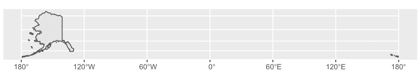
The root cause, as you no doubt have guessed, is that a part of the Alaska archipelago crosses the antimeridian.

sf::st_crop() will be your friend here, and you can apply it either in original CRS (your limits look metric and the plot has the look of the Web Mercator, which is the CRS of the popular Kontur dataset, but I speculate here) or in WGS 84 (= decimal degrees).

But you have to set the limits in units your object understands = to apply a degree based crop you must have your object in degree based CRS. Or use a meters crop for a metric CRS. A slight complication is that metric coordinates are so unfamiliar, and decimal degrees so familiar, that {ggplot2} likes to annotate even metric plots by decimal degrees. A confusion we must live with.

To get your object from one CRS to another sf::st_transform() is your friend.

[technocrat]

Consider using a more friendly projection. It's getting late for me, so I haven't done the boundary multipolygon overlay. Just code and image of plot, too long running for reprex. You might also consider binning population to create a discrete scale.

require(ggplot2)
require(sf)
# https://data.humdata.org/dataset/kontur-population-united-states-of-america?
boundaries <- st_read("/Users/ro/projects/demo/kontur_boundaries_US_20220407.gpkg")
population <- st_read("/Users/ro/projects/demo/kontur_population_US_20220630.gpkg")

# identify source data projection
st_crs(boundaries)[1]
st_crs(population)[1]
# Mercator type projections are distorted
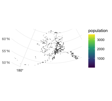
# consider changing to NAD83, Alaska Albers
# https://epsg.io/3338
boundaries <- st_transform(boundaries, 3338)
population <- st_transform(population, 3338)

# subset out alaska boundary
alaska <- boundaries[which(boundaries$name_en == "Alaska"),]

# subset out alaska population
ak_pop <- population[st_intersects(alaska,population)[1][[1]],]

# plot

ggplot(ak_pop) + 
  geom_sf(aes(fill = population)) +
  scale_fill_continuous(type = "viridis") +
  theme_minimal()