Hey, am new to R Studio. Apart from Tidyverse, Skimr, Janitor. Which other packages do you recommend I install mostly for test of statistics (inferential statistics).
All the standard (classic) methods are already included by default in the {stats} package. For a listing
help("stats")
1 Like
Thank you very much, I have seen it. But the problem am having is their syntax.
I used "?" to get details about the syntax
Like
? Chisq.test
But the example they give isn't that clear.
When I was first learning to use R (no one actually learns R —there's way too much to look at, let alone understand and remember), I grumbled that help() needed its own help("help"). And then I found it and discovered that in order to understand help("help") you must first understand help.
So, here's my epiphany—I already knew how to do this from 1963, when I took school algebra: f(x) = y, which are three objects.
In a way that's trivial,, because in R everything is an object, including objects that contain other objects. And, crucially, functions, too, as in f(g(x) = y. All objects have attributes, like being character or numeric typeof or, in the case of functions, the attribute of transforming one object into another.
The one object is conventionally called x, which is something to hand, and x is provided as an argument to f. To be prissy about it, in the definition of f, x is a parameter or formal argument, but outside of the TA's hearing no one will complain if you use just "argument." The result of f(x) is the value of the function, which you may also remember as its return value.
f may take multiple arguments, such as $lm(mpg ~ drat, data = mtcars) when doing linear regression. The help("some_function") displays the usage compactly using a standard presentation. Here's an example.
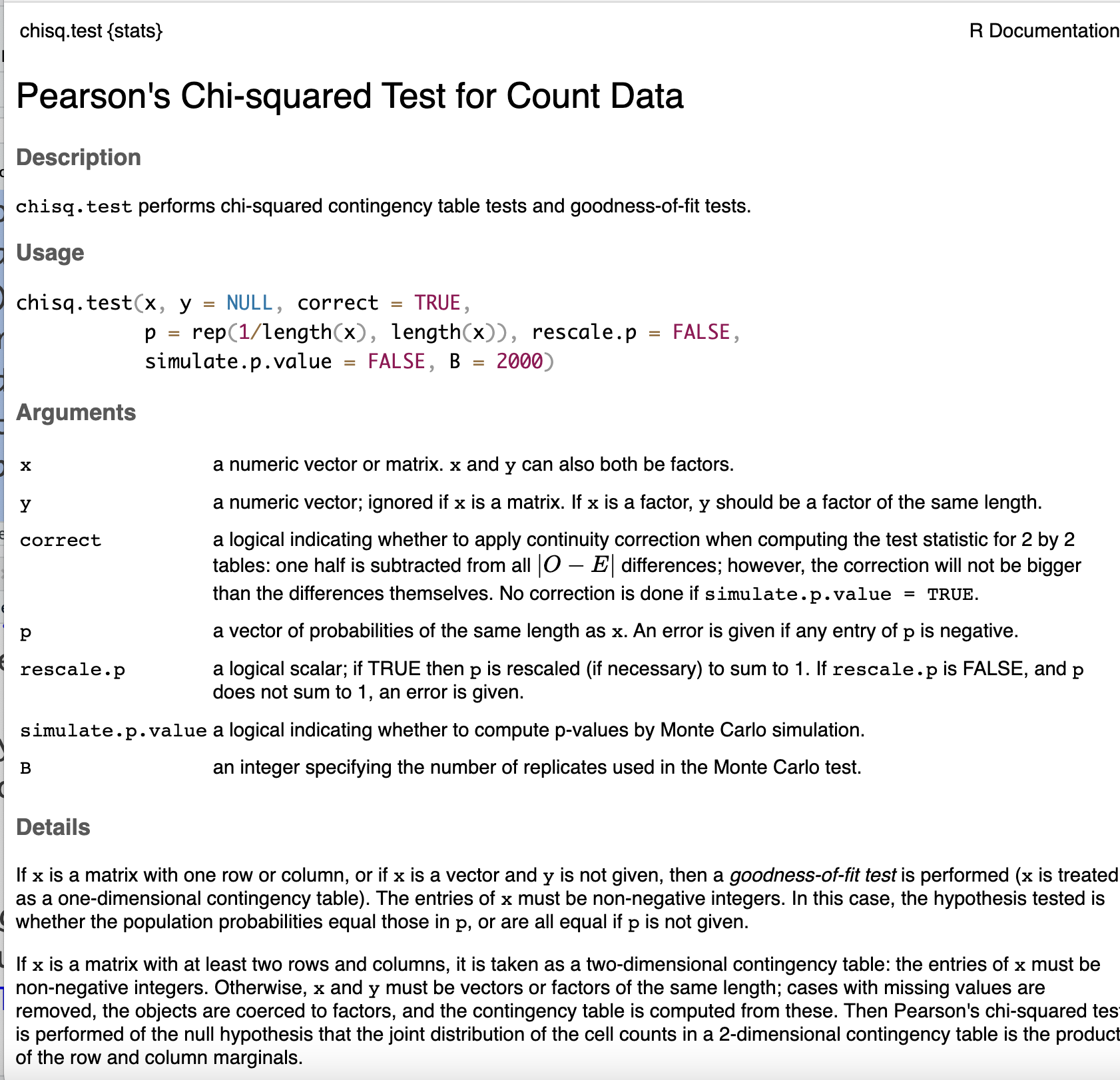
At the very top is the name of the function, followed by its package name in curly braces, in this case chisq.test{stats}, then a fancy title Pearson's Chi-squared Test for Count Data, followed by Usage. This is the crucial part because it contains the function signature
Usage
chisq.test(x, y = NULL, correct = TRUE,
           p = rep(1/length(x), length(x)), rescale.p = FALSE,
           simulate.p.value = FALSE, B = 2000)
Here is the function with its seven arguments. *All of the arguments with an equal sign = have defaults and do not need to be entered. So, to begin, this is just chisq.test(x) and the others will be assumed automatically.
The next section, Arguments describes what is needed for each argument. In this case, we focus on x, since we can rely on defaults for the rest for the time being.
x
a numeric vector or matrix.xandycan also both be factors.
Let's stop here and try something
chisq.test(1:30)
The syntax is simply the name of f, which is chisq.test and the argument, which is shorthand for the vector of integers 1 through 30 and enclosed by `(). But we knew this long ago from f(x) = y. Syntax is easy; if we are using a y argument in addition, we just add it either positionally f(x,y) or by name f(x,y=y).
Usage can be harder because it's not always obvious what all the arguments are without reading the section to be sure not to give a list object as x when a vector or matrix is required and making sure that it's numeric.
The Details section provides information that is only needed if the user already knows how to use a function to perform a test and is interested in the subtleties. As statistical learning progresses, reading the section begins to provide some hazy notion of what's going on with an unfamiliar function under the hood, but at first, it may be incomprehensible.
The next section Value shows the return of f, what you can expect to be contained in the output if the function gets the type of argument it expects.
Source is almost never going to be of interest.
References is sometimes interesting and running the eye over can be rewarding. Agresti mentioned here is the standard text for categorical data which will be seen referenced again and again and the realization may precipitate that it would be useful seeing. (The 2018 third edition comes with R code.)
See Also
For goodness-of-fit testing, notably of continuous distributions, ks.test.
Usually just run the eye over this because it may come the rescue in cases were the Title didn't grab the attention sufficiently. The implication of the brief aside is that chisq.test is for Count data and there's this ks.test for continuous data. Often this trips me to the realization that I didn't have the proper orientation to the problem and blew the distinction being the reason results were not as expected.
Finally, Examples
Here's the first supplemented with some additional output and commentary at the end.
## From Agresti(2007) p.39
M <- as.table(rbind(c(762, 327, 468), c(484, 239, 477)))
dimnames(M) <- list(
  gender = c("F", "M"),
  party = c("Democrat", "Independent", "Republican")
)

M
#>       party
#> gender Democrat Independent Republican
#>      F      762         327        468
#>      M      484         239        477

(Xsq <- chisq.test(M)) # Prints test summary
#>
#>  Pearson's Chi-squared test
#>
#> data:  M
#> X-squared = 30.07, df = 2, p-value = 2.954e-07
Xsq$observed # observed counts (same as M)
#>       party
#> gender Democrat Independent Republican
#>      F      762         327        468
#>      M      484         239        477
Xsq$expected # expected counts under the null
#>       party
#> gender Democrat Independent Republican
#>      F 703.6714    319.6453   533.6834
#>      M 542.3286    246.3547   411.3166
Xsq$residuals # Pearson residuals
#>       party
#> gender   Democrat Independent Republican
#>      F  2.1988558   0.4113702 -2.8432397
#>      M -2.5046695  -0.4685829  3.2386734
Xsq$stdres # standardized residuals
#>       party
#> gender   Democrat Independent Republican
#>      F  4.5020535   0.6994517 -5.3159455
#>      M -4.5020535  -0.6994517  5.3159455

# full htest structure
str(Xsq)
#> List of 9
#>  $ statistic: Named num 30.1
#>   ..- attr(*, "names")= chr "X-squared"
#>  $ parameter: Named int 2
#>   ..- attr(*, "names")= chr "df"
#>  $ p.value  : num 2.95e-07
#>  $ method   : chr "Pearson's Chi-squared test"
#>  $ data.name: chr "M"
#>  $ observed : 'table' num [1:2, 1:3] 762 484 327 239 468 477
#>   ..- attr(*, "dimnames")=List of 2
#>   .. ..$ gender: chr [1:2] "F" "M"
#>   .. ..$ party : chr [1:3] "Democrat" "Independent" "Republican"
#>  $ expected : num [1:2, 1:3] 704 542 320 246 534 ...
#>   ..- attr(*, "dimnames")=List of 2
#>   .. ..$ gender: chr [1:2] "F" "M"
#>   .. ..$ party : chr [1:3] "Democrat" "Independent" "Republican"
#>  $ residuals: 'table' num [1:2, 1:3] 2.199 -2.505 0.411 -0.469 -2.843 ...
#>   ..- attr(*, "dimnames")=List of 2
#>   .. ..$ gender: chr [1:2] "F" "M"
#>   .. ..$ party : chr [1:3] "Democrat" "Independent" "Republican"
#>  $ stdres   : 'table' num [1:2, 1:3] 4.502 -4.502 0.699 -0.699 -5.316 ...
#>   ..- attr(*, "dimnames")=List of 2
#>   .. ..$ gender: chr [1:2] "F" "M"
#>   .. ..$ party : chr [1:3] "Democrat" "Independent" "Republican"
#>  - attr(*, "class")= chr "htest"
Created on 2023-04-29 with reprex v2.0.2
Map this back to the signature function.
M is a table object (also called a contingency table) that plays the role of x as the first argument. A value piece of incidental intelligence is that a table also qualifies as a matrix.
The return of chisq.test(M) gives a summary of the results of the test, and other pieces can be picked out using the $ operator.
Big HOWEVER what this does not do is clearly to explain when you should use the test, what the test statistic represents and the null hypothesis that is evaluated. While it may be possible to learn statistics by using R without statistic texts and other instructional materials, it's definitely the hard way to go about it.
For that, there are several useful resources. One I like is Introductory Statistics with R, 2d ed. by Peter Dalgaard. Its's pitched at students without a math background who need to use statistics in research. The author is a member of the R Core Development Team, which is kind of a big deal.
2 Likes
Thank you very much sir for your contribution...
I love the way you simplify everything, from the syntax, Argument, value and the example.
Am grateful.
Thank you very much sir...
1 Like
Is it possible to transform M object to dataframe, but "as is" ?
When I do:
M %>% as.data.frame()
it adds Freq column and changes the layout of M which I do not want.
Do you mean
M <- as.table(rbind(c(762, 327, 468), c(484, 239, 477)))
dimnames(M) <- list(
  gender = c("F", "M"),
  party = c("Democrat", "Independent", "Republican")
)

(M |> data.frame())[-3]
#>   gender       party
#> 1      F    Democrat
#> 2      M    Democrat
#> 3      F Independent
#> 4      M Independent
#> 5      F  Republican
#> 6      M  Republican
(which doesn't look very useful) or
M <- as.table(rbind(c(762, 327, 468), c(484, 239, 477)))
dimnames(M) <- list(
  gender = c("F", "M"),
  party = c("Democrat", "Independent", "Republican")
)

M |> as.data.frame.matrix()
#>   Democrat Independent Republican
#> F      762         327        468
#> M      484         239        477
The second is much closer to my desire output, thank you, but not to mess here I just have opened a new post:
https://forum.posit.co/t/how-to-change-headers-of-rows-and-columns/165335
1 Like
This topic was automatically closed 7 days after the last reply. New replies are no longer allowed.
If you have a query related to it or one of the replies, start a new topic and refer back with a link.