Color stripchart according to column (3 objects)

millie_coward · November 18, 2022, 11:17am

Hi! I've put this on my normal reddit forum but no help there so I thought id try here!

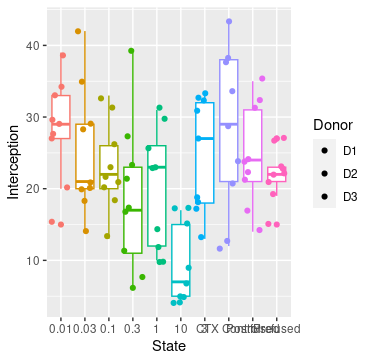
I have overlayed a stripchat onto my box & whisker, looks beautiful. But all the points are one colour when actually they're samples from 3 different donors: D1, D2 and D3 seperated in the .csv as a column called "Donor.

My Box and Whisker is Interception~State, two separate variables.

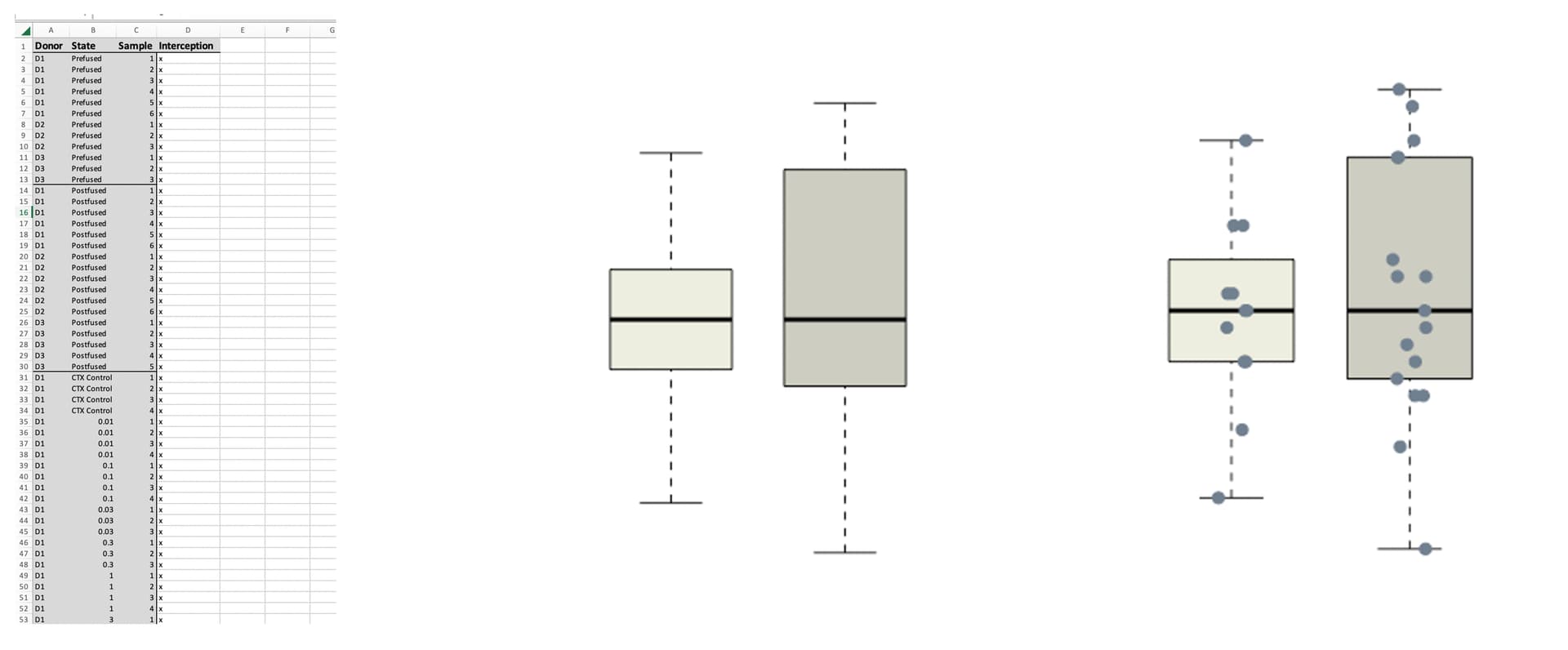
I have attached a picture of my excel (points replaced with x), a sample bar with and without the scatter.

My R Script reads:
boxplot (Interception~State, data=data.CTXScreen,
xlab="Sample State, including CTX treatment (µM)",
ylab = expression('Fibre Midline Interception'), main="Fibre Midline Interception for each state",
cex.main=2.5,
cex.lab=1.5,
cex.axis=1,
boxwex=0.7,
col= c('ivory2', 'ivory3', 'red1', 'darkorange', 'yellow', 'springgreen4', 'dodgerblue1', 'purple4', 'purple1', 'deeppink'))

stripchart(Interception~State, data=data.CTXScreen,
method = "jitter",
pch = 19,
col = c('slategrey'),
vertical = TRUE, add = TRUE)

I've been messing around attempting things like this:
V2=runif(data.CTXScreen$Donor == "D1") {col = c('slategrey')}
else if (data.CTXScreen$Donor == "D2") {col = c('dark grey')}
else (data.CTXScreen$Donor == "D3") {col = c('black')}

x <- if(data.CTXScreen$Donor == "D1") {col = c('slategrey')}
y <- if (data.CTXScreen$Donor == "D2") {col = c('darkgrey')}
z <- if (data.CTXScreen$Donor == "D3") {col = c('black')}

df = data.frame(V1=runif(Donor == "D1", col = c('slategrey')), V2=runif(Donor == "D2", col = c('darkgrey')), V3=runif(Donor == "D3", col = c('black')))

df = data.frame(V1=sample.int(Donor == "D1", col = c('slategrey'), replace=TRUE), V2=runif(Donor == "D2", col = c('darkgrey')), V3=runif(Donor == "D3", col = c('black')))

Overall a very big mess and I wonder if anyone could give me a hand. I feel like its such a simple issue, but its had me stumped since about August!

This post is most helpful but I just can't see to translate it to my script

jrkrideau · November 21, 2022, 11:44pm

I think we need some sample data. A handy way to supply some sample data is the dput() function. In the case of a large dataset something like dput(head(mydata, 100)) should supply the data we need.

millie_coward · November 22, 2022, 8:25am

Hi! I can't actually display my data online, hence why I blocked it out. I have attached on this thread a picture of what the columns look like and the data runs from 1-50, does that help?

jrkrideau · November 22, 2022, 12:30pm

Noat really. It is pretty close to unreadable. If you cannot upload the data for reasons of confidentiality can you create and upload a simulated dataset. Generally it does not matter what the actual sample data is as long as it is in the same format.

This usually means that if you do an `str(mydata) where mydata is the name of your data, the results are the same as str(my_sample_data by which I mean the variadle types are the same. Simple example: The key poinnt is that the data types are the same. Here they are all intigers.

'data.frame':	5 obs. of  3 variables:
 $ aa: int  1 4 7 10 13
 $ bb: int  2 5 NA 11 14
 $ cc: int  3 6 9 12 NA

jrkrideau · November 22, 2022, 2:52pm

Could you supply that data in dput format, please.

Using my tiny example it should look like this.

dput(dat1)
structure(list(Pre_fog = c(4.94, 5.24, 4.8, NA, NA), Fog = c(5.54, 
5.44, 5.32, 5.53, 5.54), Post_fog = c(4.86, 4.97, 4.59, 4.77, 
NA)), row.names = c(NA, 5L), class = "data.frame")

This gives us an exact cpy of your data.

Thanks.

millie_coward · November 22, 2022, 3:05pm

structure(list(Donor = structure(c(1L, 1L, 1L, 2L, 2L, 2L, 3L, 
3L, 3L, 1L, 1L, 1L, 2L, 2L, 2L, 3L, 3L, 3L, 1L, 1L, 1L, 1L, 1L, 
1L, 1L, 1L, 1L, 1L, 1L, 1L, 1L, 1L, 1L, 1L, 1L, 1L, 1L, 1L, 1L, 
1L, 1L, 1L, 2L, 2L, 2L, 2L, 2L, 2L, 2L, 2L, 2L, 2L, 2L, 2L, 2L, 
2L, 2L, 2L, 2L, 2L, 2L, 2L, 2L, 2L, 2L, 2L, 3L, 3L, 3L, 3L, 3L, 
3L, 3L, 3L, 3L, 3L, 3L, 3L, 3L, 3L, 3L, 3L, 3L, 3L, 3L, 3L, 3L, 
3L, 3L, 3L), .Label = c("D1", "D2", "D3"), class = "factor"), 
    State = structure(c(10L, 10L, 10L, 10L, 10L, 10L, 10L, 10L, 
    10L, 9L, 9L, 9L, 9L, 9L, 9L, 9L, 9L, 9L, 8L, 8L, 8L, 1L, 
    1L, 1L, 3L, 3L, 3L, 2L, 2L, 2L, 4L, 4L, 4L, 5L, 5L, 5L, 7L, 
    7L, 7L, 6L, 6L, 6L, 8L, 8L, 8L, 1L, 1L, 1L, 2L, 2L, 2L, 3L, 
    3L, 3L, 4L, 4L, 4L, 5L, 5L, 5L, 7L, 7L, 7L, 6L, 6L, 6L, 8L, 
    8L, 8L, 2L, 2L, 2L, 1L, 1L, 1L, 3L, 3L, 3L, 4L, 4L, 4L, 5L, 
    5L, 5L, 7L, 7L, 7L, 6L, 6L, 6L), .Label = c("0.01", "0.03", 
    "0.1", "0.3", "1", "10", "3", "CTX Control", "Postfused", 
    "Prefused"), class = "factor"), Sample = c(1L, 2L, 3L, 1L, 
    2L, 3L, 1L, 2L, 3L, 1L, 2L, 3L, 1L, 2L, 3L, 1L, 2L, 3L, 1L, 
    2L, 3L, 1L, 2L, 3L, 1L, 2L, 3L, 1L, 2L, 3L, 1L, 2L, 3L, 1L, 
    2L, 3L, 1L, 2L, 3L, 1L, 2L, 3L, 1L, 2L, 3L, 1L, 2L, 3L, 1L, 
    2L, 3L, 1L, 2L, 3L, 1L, 2L, 3L, 1L, 2L, 3L, 1L, 2L, 3L, 1L, 
    2L, 3L, 1L, 2L, 3L, 1L, 2L, 3L, 1L, 2L, 3L, 1L, 2L, 3L, 1L, 
    2L, 3L, 1L, 2L, 3L, 1L, 2L, 3L, 1L, 2L, 3L), NucleiCount = c(984L, 
    474L, 901L, 582L, 780L, 1015L, 501L, 1202L, 438L, 1271L, 
    1055L, 1322L, 2022L, 1954L, 1967L, 2323L, 2243L, 1494L, 1507L, 
    1386L, 1351L, 1506L, 1261L, 1356L, 1051L, 1292L, 1234L, 1503L, 
    1258L, 1542L, 645L, 676L, 1326L, 1245L, 1422L, 1355L, 1207L, 
    1240L, 1205L, 1064L, 1077L, 1229L, 1770L, 1768L, 1740L, 2227L, 
    2117L, 2039L, 2008L, 1927L, 1965L, 1965L, 2162L, 2046L, 1873L, 
    1602L, 1463L, 1884L, 2133L, 2095L, 2169L, 2344L, 2173L, 2465L, 
    2697L, 722L, 2064L, 1988L, 1826L, 1996L, 1916L, 2164L, 2030L, 
    1916L, 2231L, 2097L, 2160L, 2198L, 2152L, 1918L, 1614L, 2211L, 
    2128L, 1965L, 2204L, 2288L, 2425L, 529L, 34L, 504L), Interception = c(15L, 
    21L, 22L, 19L, 23L, 27L, 22L, 27L, 23L, 31L, 17L, 14L, 24L, 
    24L, 21L, 35L, 32L, 22L, 29L, 13L, 24L, 27L, 15L, 29L, 21L, 
    20L, 13L, 21L, 14L, 35L, 11L, 8L, 6L, 14L, 12L, 10L, 18L, 
    13L, 19L, 4L, 7L, 15L, 34L, 43L, 38L, 33L, 30L, 39L, 42L, 
    20L, 28L, 22L, 33L, 18L, 21L, 17L, 39L, 23L, 26L, 23L, 33L, 
    17L, 33L, 9L, 17L, 5L, 21L, 38L, 12L, 18L, 20L, 29L, 28L, 
    20L, 34L, 23L, 31L, 26L, 17L, 27L, 23L, 31L, 10L, 30L, 32L, 
    31L, 27L, 17L, 5L, 4L), Diameter = c(22.7542, 28.9521, 17.7549, 
    13.924, 22.839, 25.471, 32.6029, 23.9566, 38.461, 28.6973, 
    38.461, 44.1495, 26.4049, 33.0272, 25.8106, 27.8483, 24.4521, 
    26.4048, 32.1783, 31.5839, 33.5367, 28.8671, 30.8199, 37.0176, 
    53.2342, 35.8292, 35.3195, 39.7348, 41.178, 39.3101, 23.2634, 
    19.6977, 12.387, 16.5561, 20.1222, 21.4806, 17.7447, 21.8203, 
    11.0372, 13.4146, 18.0845, 15.2826, 28.3575, 24.1975, 26.398, 
    21.141, 26.5747, 24.0276, 30.8199, 20.8014, 29.1218, 29.1387, 
    27.6944, 21.3958, 25.471, 24.2114, 24.8412, 16.1317, 14.0089, 
    19.1882, 14.0088, 16.3013, 11.5467, 15.7072, 16.8108, 19.7826, 
    21.1409, 26.405, 23.0938, 21.3955, 24.3672, 21.5655, 19.0293, 
    14.9429, 19.2731, 21.4806, 20.9711, 23.6881, 20.8863, 21.3108, 
    24.0277, 14.943, 14.179, 14.6034, 11.8013, 9.6787, 10.9521, 
    9.1692, 5.4337, 9.4243)), class = "data.frame", row.names = c(NA, 
-90L)) ```

millie_coward · November 22, 2022, 3:06pm

'data.frame':	90 obs. of  6 variables:
 $ Donor       : Factor w/ 3 levels "D1","D2","D3": 1 1 1 2 2 2 3 3 3 1 ...
 $ State       : Factor w/ 10 levels "0.01","0.03",..: 10 10 10 10 10 10 10 10 10 9 ...
 $ Sample      : int  1 2 3 1 2 3 1 2 3 1 ...
 $ NucleiCount : int  984 474 901 582 780 1015 501 1202 438 1271 ...
 $ Interception: int  15 21 22 19 23 27 22 27 23 31 ...
 $ Diameter    : num  22.8 29 17.8 13.9 22.8 ... ```

jrkrideau · November 22, 2022, 4:09pm

Excellent, thank you.

I am just on my way out so will not have a chance to do anything for a few hours at least but is good to get the data.

jrkrideau · November 22, 2022, 5:23pm

I was a bit early so I had a few minutes to play with this. I suddenly realised that I had not used Base R graphics in years so I gave it a try in ggplot2

I have renamed your dataset dat1 to save some typing and tried this.

library(ggplot2)
ggplot(dat1, aes(State, Interception, fill = State)) + geom_boxplot() +
  geom_jitter(aes(colour = Donor)) +
  guides(fill = FALSE)

Does it come anywhere near to doing what you want?

It occurs to me that the stripchart might benefit by using different plotting shapes.

millie_coward · November 22, 2022, 5:42pm

I've had some trouble downloading ggplot on my R, so I am looking for a way to do it without it. I saw this post did it with baseR: Color points according to column - #5 by nirgrahamuk (but his points were numeric, where as mine are each point associated with a non-numeric label, if that makes sense)

Sorry I know that adds another layer of problem solving, but I thought I may be able to do it without ggplots, maybe using objects and data frames instead? Which is what I tried (in the original post). I may just have to troubleshoot my ggplot download if not!

jrkrideau · November 22, 2022, 9:11pm

Okay.

install.packages("ggplot2")

should do it though it is probably better to do an

install.packages("tidyverse")

is likely better as it installs a number of useful packages.

In the meantime I'll have a look at what @ nirgrahamuk did.

Meanwhile this is as far as I have gotten.
box1

millie_coward · November 23, 2022, 8:58am

That looks gorgeous! Just need to colour the points!

ggplot2 and tidyverse won't download on my R, I get errors on my source packages which look like this:

  installation of package ‘scales’ had non-zero exit status
* installing *source* package ‘vctrs’ ...
** package ‘vctrs’ successfully unpacked and MD5 sums checked
** libs
xcrun: error: invalid active developer path (/Library/Developer/CommandLineTools), missing xcrun at: /Library/Developer/CommandLineTools/usr/bin/xcrun
ERROR: compilation failed for package ‘vctrs’ ```

I have a workshop today so can't troubleshoot it during the day. Will have a look tonight but it's caused a lot of frustration for me this morning! I can't even seem to download the Xcode either. I will work it out!

nirgrahamuk · November 23, 2022, 10:43am

as a macOS user you if you are installing a package from source rather than a binary; it will require compilation; This means you need the correct tooling on your system (outside of R)

install Xcode in your system (not in R) and the recommended development tools for macOS systems.
https://mac.r-project.org/tools/

jrkrideau · November 23, 2022, 12:42pm

Try this

library(ggplot2)
ggplot(dat1, aes(State, Interception, fill = State)) + geom_boxplot() +
  geom_jitter(aes(colour = Donor)) +
  guides(fill = FALSE)

jrkrideau · November 23, 2022, 4:09pm

I think I have outsmarted myself. I think I have a decent layout for @ millie_coward's plot. See

library(ggplot2)

ggplot(dat1, aes(State, Interception, colour = State)) + geom_boxplot() +
    geom_jitter(aes(colour = Donor)) + 
     guides(colour  = "none")

I do not seem to be able to use fill = with a geom_points() command . The geom_jitter() command is just version of it. Unfortunately guides(colour = "none") takes out both legends. Definitely I do not want the boxplot() legend.

Can anyone suggest a solution? I suspect I am missing something obvious here.

jrkrideau · November 23, 2022, 4:48pm

[quote="jrkrideau, post:16, topic:153051"]
I think I have outsmarted myself.

I may be making some progress. I think I have a working graph


library(ggplot2)

mycols  <- c("#1B9E77", "#D95F02", "#7570B3", "#E7298A", "#66A61E", "#E6AB02", "#A6761D", 
             "#666666", "#1B9E77", "#D95F02", "#7570B3", "#E7298A", "#66A61E")

p1  <- ggplot(dat1, aes(State, Interception, colour = State)) + 
          geom_boxplot() +
          geom_jitter(aes(colour = Donor)) + 
         guides(colour  = "none") +
          annotate(geom="text", x = 10, y=45, label="Donor 1", color="#1B9E77") +
          annotate(geom="text", x = 10, y=44, label="Donor 2", color="#D95F02") +
          annotate(geom="text", x = 10, y=43, label="Donor 2", color="#7570B3")

p1 +   scale_color_manual(values= mycols)

millie_coward · November 23, 2022, 7:31pm

* DONE (ggplot2)

The downloaded source packages are in
	‘/private/var/folders/gf/d8fbbk2n2h92rrhmywp8dj5h0000gn/T/RtmpLi9YJc/downloaded_packages’ ```

millie_coward · November 23, 2022, 7:49pm

just ran it and you sir are a genius! looks gorgeous!!!!!!!!

I would love to understand what all of it means though?

mycols <- c("#1B9E77", "#D95F02", "#7570B3", "#E7298A", "#66A61E", "#E6AB02", "#A6761D", "#666666", "#1B9E77", "#D95F02", "#7570B3", "#E7298A", "#66A61E")

this is colours used in the graphs? all of them? but why 13 different colours?

then..

aes(colour = Donor)) + guides(colour = "none") +

aes is associating something with something else? so colour with donor.. v cool, but what's the guide part? "none"? I wonder what that means?

then next question..

annotate(geom="text", x = 10, y=45, label="Donor 1", color="#1B9E77") +
annotate(geom="text", x = 10, y=44, label="Donor 2", color="#D95F02") +
annotate(geom="text", x = 10, y=43, label="Donor 2", color="#7570B3")

^ all of this is.. just doing the top right labels? so is the aes where you associate colours with data points ono the stripchart?

I shall merge it in with my script but I would love to understand a breakdown of the code if you have time, if not no worries I will work it out & big thank you from the bioengineering field!

jrkrideau · November 23, 2022, 11:32pm

The State variable has 13 values and we need an entry for each one. You can use any mix of colours that you want but you need 13 entries. Except that it would screw up the **colour = Donor ** coding you could code them all "red" as long as there are 13.
You may want to play around with the colours to get a better mix .

I just hijacked a set of colours from a RColorBrewer palate and duplicated a few entries to get 13. I realise this sounds like gibberish but it does make sense if you know a bit about ggplot2.

all of this is.. just doing the top right labels? so is the aes where you associate colours with data points onto the stripchart?

Yes, I am assuming that ggplot is cycling through the mycols so I have assigned the first three colours to the "legend" since it should be using them to colour the dots.

There is one other thing I think we need---assuming I can figure out how to do it---and that is the Donor points should have three different symbols to differentiate them for anyone who is colourblind. It is just better practice anyway. With luck I should get a chance to have a shot at it tomorrow.

The colour command is telling ggplot to split the points into three sequences by Donor just as colour = Stateis telling the boxplot command to plot the 13 box & whisker plots.

The guides(colour = "none") is telling that we do not want any legends. Otherwise we would get a legend for States that is both redundant and looks horrible. I could not figure out a way to just get rid of the States legend and keep the Donor one so I killed both and stuck the equivalent of the "Donor" one in the body of the plot.

^ all of this is.. just doing the top right labels?

Yes, there may be a cleaner way to do it but it seems to work.

You might want to have a quick look at ggplot2: elegant graphics for data analysis. I read the 1st edition and it was quite useful until I poured a glass of Coca Cola over it and glued all the pages together.

Matthias · November 24, 2022, 9:25am

Maybe indeed this solution is a bit overcomplicated.
First of all: Do you need the boxplots to be colored as well? If not you can leave them grey (option 1), or colour their fill (option 2) so you can use the "colour = Donor" for the points.
Second. When combining boxplots with geom_jitter() you always risk to show the outlier twice. Here you can either hide the outliers, use another shape, or (as I prefer) use an alternative to jitter, geom_beeswarm, which only distributes points in width if they would overlap otherwise. (option 3) this usually "hides" the outlier points. (well not for prefused)
Finally you could use another point shape, so you have the fill argument to use, so fill and colour don't collide anymore. (option 4).

# Version 1 - boxplots in grey
ggplot(dat1, aes(State, Interception)) + 
  geom_boxplot(colour = "grey40") +
  geom_jitter(aes(colour = Donor),
              height = 0,  # Attention: Don't jitter the height! 
              size  =3) + 
  theme_bw() + 
  theme(axis.text.x = element_text(angle = 45, hjust = 1))  +
  labs(title = "Option 1")


# Version 2 - use fill for the boxplots
ggplot(dat1, aes(State, Interception)) + 
  geom_boxplot(aes(fill = State),
               show.legend = FALSE,
               alpha = 0.3) +
  geom_jitter(aes(colour = Donor),
              height = 0,  # Attention: Don't jitter the height! 
              size = 3) + 
  theme_bw() + 
  theme(axis.text.x = element_text(angle = 45, hjust = 1)) +
  labs(title = "Option 2")


# Version 3 - with beeswarm 
library(ggbeeswarm)
ggplot(dat1, aes(State, Interception)) + 
  geom_boxplot(aes(fill = State),
               show.legend = FALSE,
               alpha = 0.3) +
  ggbeeswarm::geom_beeswarm(aes(colour = Donor),
              size = 3, cex = 2, method = "center") + 
  theme_bw() + 
  theme(axis.text.x = element_text(angle = 45, hjust = 1)) +
  labs(title = "Option 3")


# Version 4 - with colour as fill
ggplot(dat1, aes(State, Interception)) + 
  geom_boxplot(aes(colour = State),
               show.legend = FALSE) +
  geom_jitter(aes(fill = Donor),
              size = 3,
              height = 0,  # Attention: Don't jitter the height! 
              shape = 21,     # shape 21 can has a fill colour! 
              colour = "grey50") +  # colour for the outline
  theme_bw() + 
  theme(axis.text.x = element_text(angle = 45, hjust = 1)) +
  labs(title = "Option 4")