Found a {ggplot2} solution that will solve the basic problem. I don't know how much embellishment you need in terms of labels, light weight, color, title, caption, font, etc.
# Install the package as follows:
# Enable the r-universe repo
options(repos = c(
fawda123 = 'https://fawda123.r-universe.dev',
CRAN = 'https://cloud.r-project.org'))
# install.packages("ggord") first
library(ggord)
library(ggplot2)
library(patchwork)
library(scales)
library(vegan)
#> Loading required package: permute
#> Loading required package: lattice
#> This is vegan 2.6-4
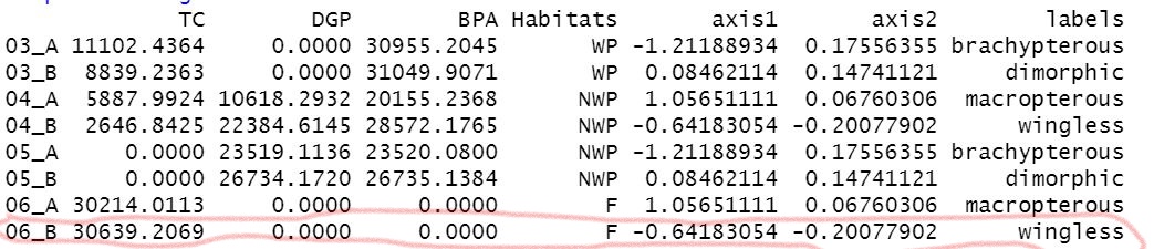
d <- data.frame(
station = c(
"03_A", "03_B", "04_A", "04_B", "05_A",
"05_B", "06_A", "06_B", "11_A", "11_B", "12_A", "12_B", "13_A",
"13_B", "14_A", "14_B", "15_A", "15_B", "16_A", "17_A", "17_B",
"19_A", "19_B", "20_A", "20_B", "21_A", "21_B", "22_A", "22_B"
), brachypterous = c(
80, 76, 56, 48, 28, 7, 16, 10, 42,
74, 23, 16, 52, 62, 79, 74, 76, 58, 26, 16, 72, 44,
27, 73, 33, 66, 55, 34, 6
), dimorphic = c(
53, 52, 70,
57, 53, 50, 68, 79, 67, 16, 48, 53, 42, 2, 71, 20,
53, 64, 18, 75, 74, 34, 6, 18, 20, 13, 20, 51, 44
), macropterous = c(
64, 11, 2, 59, 14, 76, 2, 74, 48,
70, 62, 51, 17, 67, 29, 64, 2, 58, 61, 79, 18, 63,
71, 43, 50, 11, 34, 3, 50
), wingless = c(
59, 69, 30,
35, 9, 7, 65, 63, 48, 3, 43, 27, 30, 35, 34, 57,
57, 10, 65, 7, 21, 64, 12, 29, 35, 66, 27, 4, 54
), hygrophilic = c(
54, 77, 19, 39, 70, 28, 73, 26, 39,
9, 57, 12, 34, 25, 43, 8, 59, 72, 55, 15, 23, 58,
61, 49, 45, 41, 41, 57, 76
), mesophilic = c(
49, 78,
69, 32, 77, 21, 30, 40, 6, 38, 56, 56, 40, 77, 77,
79, 39, 41, 14, 52, 69, 54, 27, 61, 33, 69, 53, 38,
78
), mesophilic_hygrophilic = c(
15, 35, 7, 13, 8, 14,
23, 34, 30, 4, 12, 20, 16, 43, 10, 32, 40, 37, 8,
32, 31, 40, 34, 42, 14, 33, 6, 27, 21
), xerophilic = c(
33,
0, 20, 31, 46, 22, 24, 49, 16, 36, 24, 20, 28, 20,
4, 31, 32, 39, 27, 48, 8, 47, 4, 23, 45, 3, 9, 26,
48
), steno_hygrophilic = c(
28, 8, 40, 40, 19, 11, 17,
13, 24, 21, 37, 42, 34, 5, 39, 8, 28, 24, 33, 39,
11, 50, 47, 11, 20, 0, 10, 32, 42
), imago = c(
20, 42,
49, 24, 29, 47, 4, 14, 27, 11, 15, 33, 18, 5, 2,
36, 26, 24, 26, 25, 31, 13, 17, 29, 47, 36, 41, 21,
18
), larva = c(
19, 38, 28, 32, 1, 45, 6, 44, 6, 31,
28, 30, 18, 41, 47, 41, 8, 12, 25, 16, 1, 24, 35,
19, 34, 50, 48, 37, 41
), larva_imago = c(
32, 23, 28,
13, 26, 28, 26, 37, 35, 15, 34, 22, 20, 45, 41, 11,
12, 4, 6, 28, 25, 21, 49, 47, 34, 3, 10, 15, 8
),
indefinite.stage = c(
33, 18, 48, 50, 33, 7, 28, 14,
46, 47, 40, 38, 25, 31, 29, 24, 33, 23, 33, 3,
30, 17, 45, 8, 43, 45, 38, 4, 46
), eurytope = c(
22,
10, 44, 28, 35, 20, 39, 36, 25, 46, 37, 13, 32,
5, 3, 31, 19, 34, 47, 32, 32, 7, 21, 34, 49,
42, 24, 3, 38
), stenotope = c(
48, 21, 4, 33, 14,
5, 0, 13, 27, 42, 2, 23, 15, 50, 5, 10, 29, 48,
45, 13, 31, 43, 25, 48, 0, 42, 19, 20, 17
), e_s = c(
4,
3, 1, 0, 3, 3, 1, 1, 4, 3, 3, 4, 5, 2, 1, 5,
1, 5, 3, 2, 5, 2, 5, 2, 0, 4, 5, 3, 5
), taille_moy = c(
19,
20, 9, 11, 12, 20, 18, 19, 14, 20, 8, 17, 15,
13, 8, 17, 14, 8, 14, 12, 8, 16, 8, 11, 20, 20,
14, 14, 15
), TC = c(
4660, 1654, 19106, 26431, 13204,
24831, 17754, 22748, 2163, 11506, 3189, 4757, 27349,
30400, 3196, 14038, 184, 9439, 4064, 6883, 24972,
25949, 30463, 16279, 19937, 16327, 5295, 6986, 11457
), DGP = c(
22062, 22519, 25111, 1693, 10380, 22230,
24382, 29825, 20859, 28576, 9466, 6049, 15330, 19374,
6623, 3310, 1398, 18474, 24519, 19115, 26490, 10927,
26925, 29764, 3501, 21676, 20168, 28462, 20345
), BPA = c(
13494,
16681, 27239, 20931, 18060, 2631, 23919, 21235, 30760,
22211, 17583, 28510, 18622, 11243, 4379, 13354, 18665,
3927, 6417, 11786, 7016, 8220, 25047, 16044, 23967,
9521, 22494, 27038, 18741
), Habitats = c(
"WP", "WP",
"F", "NWP", "NWP", "NWP", "F", "F", "WP", "WP", "WP", "WP",
"NWP", "NWP", "F", "F", "WP", "WP", "WP", "WP", "F", "F",
"F", "WP", "WP", "F", "F", "NWP", "NWP"
)
)
# omitted non-numeric variable station
Y <- d[, c(2:4)]
# summary(Y)
# pairs(Y, panel = panel.smooth)
X <- d[, c(18, 19, 20)]
# summary(X)
# pairs(X, panel = panel.smooth)
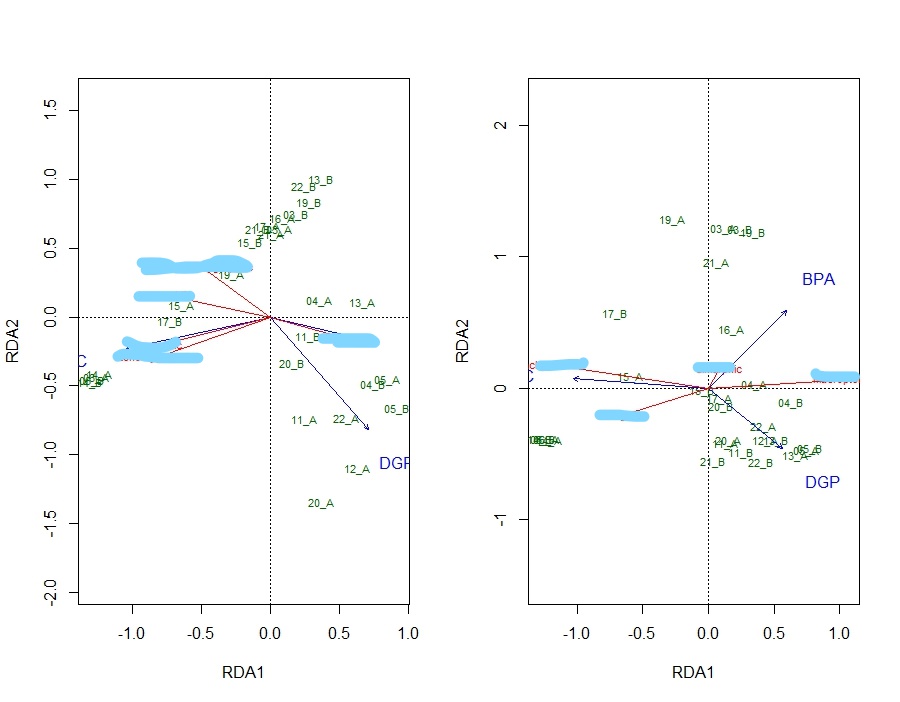
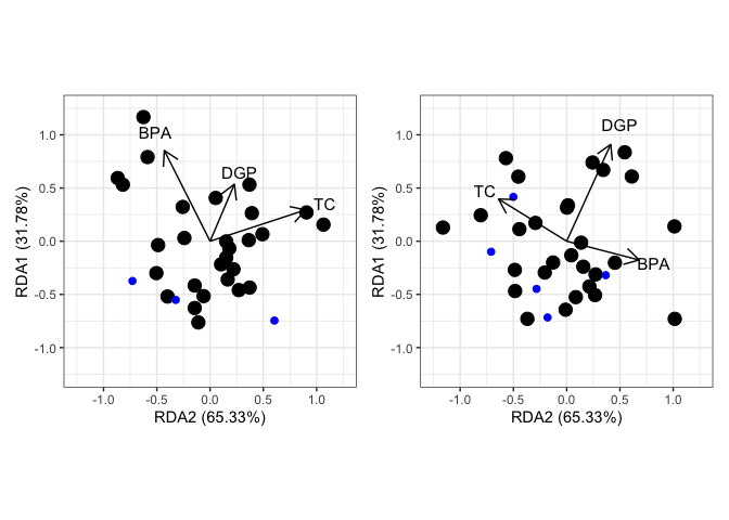
myrda <- rda(log(Y[-12, ] + 1) ~ TC + DGP + BPA, scale = TRUE, data = d[-12, ])
# anova(myrda, by = "terms")
# summary(myrda)
# Plot of Scaling 2
# wing <- plot(myrda,
# display = c("sp", "lc", "cn"),
# main = ""
# )
# spe.sc2 <- scores(myrda,
# choices = 1:2,
# display = "sp"
# )
# arrows(0, 0,
# spe.sc2[, 1] * 0.92,
# spe.sc2[, 2] * 0.92,
# length = 0,
# lty = 1, col = "red"
# )
#################################
Y1 <- d[, c(5:9)]
# summary(Y1)
# pairs(Y1, panel = panel.smooth)
X1 <- d[, c(18, 19, 20)]
# summary(X1)
# pairs(X1, panel = panel.smooth)
myrda1 <- rda(log(Y1[-12, ] + 1) ~ TC + DGP + BPA, scale = TRUE, data = d[-12, ])
# anova(myrda1, by = "terms")
# summary(myrda1)
# Plot of Scaling 2
# moisture <- plot(myrda1,
# display = c("sp", "lc", "cn"),
# main = ""
# )
# spe.sc21 <- scores(myrda1,
# choices = 1:2,
# display = "sp"
# )
# arrows(0, 0,
# spe.sc21[, 1] * 0.92,
# spe.sc21[, 2] * 0.92,
# length = 0,
# lty = 1, col = "red"
# )
# plot.new()
# par(mfrow = c(1,2))
# plot(myrda,display = c("sp", "lc", "cn"))
# plot(myrda1,display = c("sp", "lc", "cn"))
# dev.off()
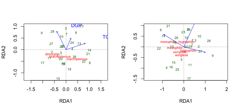
s <- summary(myrda)$concont$importance
s_x <- paste0("RDA2 (",percent(s[2], .01),")")
s_y <- paste0("RDA1 (",percent(s[5], .01),")")
s1 <- summary(myrda)$concont$importance
s1_x <- paste0("RDA2 (",percent(s[2], .01),")")
s1_y <- paste0("RDA1 (",percent(s[5], .01),")")
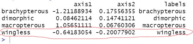
left <- ggord(myrda) +
xlim(-1.25,1.25) +
ylim(-1.25,1.25) +
xlab(s_x) +
ylab(s_y)
#> Scale for x is already present.
#> Adding another scale for x, which will replace the existing scale.
#> Scale for y is already present.
#> Adding another scale for y, which will replace the existing scale.
right <- ggord(myrda1) +
xlim(-1.25,1.25) +
ylim(-1.25,1.25) +
xlab(s1_x) +
ylab(s1_y)
#> Scale for x is already present.
#> Adding another scale for x, which will replace the existing scale.
#> Scale for y is already present.
#> Adding another scale for y, which will replace the existing scale.
left + right
Created on 2023-05-25 with reprex v2.0.2