Force ggplot2 legend to show unused categorical values?

Hello,

I have two plots with different data ranges. I want them to have the same legend with the same colors associated with their categorical variables. I am trying to force my ggplot2 legend to show categorical values that are not associated with any point. There used to be an argument called drop = FALSE in scale_color_manual but that no longer works. Does anybody know the argument to use to force ggplot2 to show unused variables in the legend?
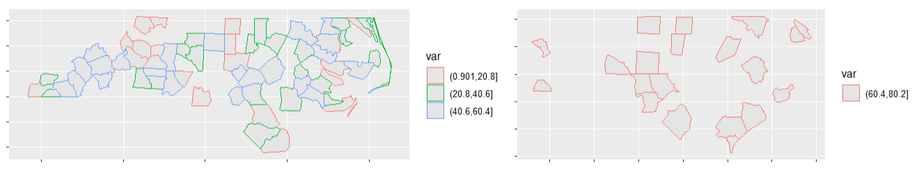
Here is my plot:

See how the legend scales are not the same?

Here is a subset of the data that I used (does not show all points):

data <- structure(list(TRANSECT = c("EAS12", "EAS12", "EMP12", "EMP17", 
"GH12", "GH17", "GH17", "GH23", "GH38", "GH38", "GH5", "GTB30", 
"MIC30"), Group = c("Cladoceran", "Cladoceran", "Rotifera", "Rotifera", 
"Rotifera", "Rotifera", "Mollusks", "Rotifera", "Rotifera", "Rotifera", 
"Rotifera", "Rotifera", "Rotifera"), DEPTH_CLASS = c("UV", "No UV", 
"UV", "UV", "No UV", "UV", "No UV", "No UV", "UV", "No UV", "No UV", 
"No UV", "UV"), Density = c(2.292795622, 72.11726105, 22025.72841, 
11004.65472, 46620.94058, 74660.99802, NA, 50434.93142, 31305.67666, 
33942.05725, 12871.3228, 20507.28229, 66078.24687), geometry = structure(list(
    structure(c(-86.4035333, 44.49025), class = c("XY", "POINT", 
    "sfg")), structure(c(-86.4035333, 44.49025), class = c("XY", 
    "POINT", "sfg")), structure(c(-86.2197667, 44.8151167), class = c("XY", 
    "POINT", "sfg")), structure(c(-86.2789333, 44.8171167), class = c("XY", 
    "POINT", "sfg")), structure(c(-86.40435, 43.059567), class = c("XY", 
    "POINT", "sfg")), structure(c(-86.458617, 43.055617), class = c("XY", 
    "POINT", "sfg")), structure(c(-86.458617, 43.055617), class = c("XY", 
    "POINT", "sfg")), structure(c(-86.539017, 43.054067), class = c("XY", 
    "POINT", "sfg")), structure(c(-86.722433, 43.060333), class = c("XY", 
    "POINT", "sfg")), structure(c(-86.722433, 43.060333), class = c("XY", 
    "POINT", "sfg")), structure(c(-86.322017, 43.074533), class = c("XY", 
    "POINT", "sfg")), structure(c(-85.4930167, 45.2598), class = c("XY", 
    "POINT", "sfg")), structure(c(-86.96095, 41.981917), class = c("XY", 
    "POINT", "sfg"))), class = c("sfc_POINT", "sfc"), precision = 0, bbox = structure(c(xmin = -86.96095, 
ymin = 41.981917, xmax = -85.4930167, ymax = 45.2598), class = "bbox"), crs = structure(list(
    input = "EPSG:4326", wkt = "GEOGCRS[\"WGS 84\",\n    ENSEMBLE[\"World Geodetic System 1984 ensemble\",\n        MEMBER[\"World Geodetic System 1984 (Transit)\"],\n        MEMBER[\"World Geodetic System 1984 (G730)\"],\n        MEMBER[\"World Geodetic System 1984 (G873)\"],\n        MEMBER[\"World Geodetic System 1984 (G1150)\"],\n        MEMBER[\"World Geodetic System 1984 (G1674)\"],\n        MEMBER[\"World Geodetic System 1984 (G1762)\"],\n        MEMBER[\"World Geodetic System 1984 (G2139)\"],\n        ELLIPSOID[\"WGS 84\",6378137,298.257223563,\n            LENGTHUNIT[\"metre\",1]],\n        ENSEMBLEACCURACY[2.0]],\n    PRIMEM[\"Greenwich\",0,\n        ANGLEUNIT[\"degree\",0.0174532925199433]],\n    CS[ellipsoidal,2],\n        AXIS[\"geodetic latitude (Lat)\",north,\n            ORDER[1],\n            ANGLEUNIT[\"degree\",0.0174532925199433]],\n        AXIS[\"geodetic longitude (Lon)\",east,\n            ORDER[2],\n            ANGLEUNIT[\"degree\",0.0174532925199433]],\n    USAGE[\n        SCOPE[\"Horizontal component of 3D system.\"],\n        AREA[\"World.\"],\n        BBOX[-90,-180,90,180]],\n    ID[\"EPSG\",4326]]"), class = "crs"), n_empty = 0L), 
    Dens_CAT = c("<10000", "<10000", "<30000", "<20000", "<50000", 
    "<80000", NA, "<60000", "<40000", "<40000", "<20000", "<30000", 
    "<70000")), class = c("sf", "grouped_df", "tbl_df", "tbl", 
"data.frame"), row.names = c(NA, -13L), groups = structure(list(
    DEPTH_CLASS = c("No UV", "UV"), .rows = structure(list(c(2L, 
    5L, 7L, 8L, 10L, 11L, 12L), c(1L, 3L, 4L, 6L, 9L, 13L)), ptype = integer(0), class = c("vctrs_list_of", 
    "vctrs_vctr", "list"))), class = c("tbl_df", "tbl", "data.frame"
), row.names = c(NA, -2L), .drop = TRUE), sf_column = "geometry", agr = structure(c(TRANSECT = NA_integer_, 
Group = NA_integer_, DEPTH_CLASS = NA_integer_, Density = NA_integer_, 
Dens_CAT = NA_integer_), class = "factor", levels = c("constant", 
"aggregate", "identity"))

Here is the code that I'm using to generate the plots


themes <- theme(axis.text.x = element_blank(),  # remove x-axis text
                axis.text.y = element_blank(), # remove y-axis text
                axis.ticks = element_blank(),  # remove axis ticks
                axis.title.x = element_text(size=18), # remove x-axis labels
                axis.title.y = element_text(size=18), # remove y-axis labels
                panel.background = element_blank(), 
                panel.grid.major = element_blank(),  #remove major-grid labels
                panel.grid.minor = element_blank(),  #remove minor-grid labels
                plot.background = element_blank(),
                legend.key.size = unit(0.25, 'cm'))

p1 <- data %>%
  filter(DEPTH_CLASS == "UV") %>%
  drop_na(Dens_CAT) %>%
  ggplot() +
  geom_sf(aes(size = Dens_CAT, color=Dens_CAT)) +
  scale_color_discrete(type = cols,
                       drop = FALSE) + # this argument does not work
  themes +
  guides(color='legend', size='legend') +
  labs(color = bquote('Indiv'~m^-3),
       size = bquote('Indiv'~m^-3))

p2 <- data %>%
  filter(DEPTH_CLASS == "No UV") %>%
  drop_na(Dens_CAT) %>%
  ggplot() +
  geom_sf(aes(size = Dens_CAT, color=Dens_CAT)) +
  scale_color_discrete(type = cols,
                       drop = FALSE)  + #this argument does not work
  themes +
  guides(color='legend', size='legend') +
  labs(color = bquote('Indiv'~m^-3),
       size = bquote('Indiv'~m^-3)) 

grid.arrange(p1,p2, nrow=1)

Any help would be greatly appreciated. Thank you so much!

Below is one way to combine and show all categorical values for two plots using the patchwork package. Unfortunately, I could not get the data to work that you shared, so I used sample data. The drop = F argument in scale_color_discrete works for me, so I'm not sure why it failed to work in your specific case.

library(tidyverse)
library(patchwork)

# sample data
nc <- sf::st_read(system.file("shape/nc.shp", package = "sf"), quiet = TRUE) |>
  mutate(var = cut(CRESS_ID, 5))

# 5 color levels for the plots
v = sort(unique(nc$var))
levels(v)
#> [1] "(0.901,20.8]" "(20.8,40.6]"  "(40.6,60.4]"  "(60.4,80.2]"  "(80.2,100]"

# 2 data subsets to plot (level 5 left off intentionally)
nc1 = nc |> filter(var %in% v[1:3])
nc2 = nc |> filter(var %in% v[4])

# plots
theme = theme(axis.text = element_blank())
g1 = ggplot(nc1) + geom_sf(aes(color = var)) + theme
g2 = ggplot(nc2) + geom_sf(aes(color = var)) + theme
# layout with 2 scales
g1 + g2

# layout with 2 scales showing all 5 categorical values
g1 + g2 & scale_color_discrete(drop = F)

# layout with consolidated scale (showing all 5 levels)
g1 + g2 + plot_layout(guides = 'collect') & scale_color_discrete(drop = F)

Created on 2023-01-19 with reprex v2.0.2.9000

What is the cols you are referring to in this call?

  scale_color_discrete(type = cols,
                       drop = FALSE)  + #this argument does not work

I don't see it declared as a variable in your code, and although there is function called cols() that lives in {readr}, which is a part of the tidyverse, it does not make sense in this context.

Having said that I believe you need to do two things:

  • declare the Dens_CAT variable as a factor before filtering to p1 and p2
  • add a scale_size_discrete with drop = FALSE, so that both legends (color and size) have the drop argument aligned.

Also note, and this is merely an observation and not a critique, that by using DEPTH _CLASS as a faceting variable you could do with a single ggplot2 call, and save yourself from having a significant amount of code twice, which is - for me at least - a nightmare to maintain.

library(tidyverse)
library(sf)

data <- structure(list(TRANSECT = c("EAS12", "EAS12", "EMP12", "EMP17", 
                                    "GH12", "GH17", "GH17", "GH23", "GH38", "GH38", "GH5", "GTB30", 
                                    "MIC30"), 
                       Group = c("Cladoceran", "Cladoceran", "Rotifera", "Rotifera",
                                 "Rotifera", "Rotifera", "Mollusks", "Rotifera", "Rotifera", "Rotifera", 
                                 "Rotifera", "Rotifera", "Rotifera"),
                       DEPTH_CLASS = c("UV", "No UV",
                                       "UV", "UV", "No UV", "UV", "No UV", "No UV", "UV", "No UV", "No UV",
                                       "No UV", "UV"), 
                       Density = c(2.292795622, 72.11726105, 22025.72841,
                                   11004.65472, 46620.94058, 74660.99802, NA, 50434.93142, 31305.67666,
                                   33942.05725, 12871.3228, 20507.28229, 66078.24687), 
                       geometry = structure(list(
                         structure(c(-86.4035333, 44.49025), class = c("XY", "POINT","sfg")),
                         structure(c(-86.4035333, 44.49025), class = c("XY", "POINT", "sfg")), 
                         structure(c(-86.2197667, 44.8151167), class = c("XY", "POINT", "sfg")),
                         structure(c(-86.2789333, 44.8171167), class = c("XY", "POINT", "sfg")),
                         structure(c(-86.404350, 43.059567), class = c("XY", "POINT", "sfg")), 
                         structure(c(-86.458617, 43.055617), class = c("XY", "POINT", "sfg")), 
                         structure(c(-86.458617, 43.055617), class = c("XY", "POINT", "sfg")), 
                         structure(c(-86.539017, 43.054067), class = c("XY", "POINT", "sfg")), 
                         structure(c(-86.722433, 43.060333), class = c("XY", "POINT", "sfg")),
                         structure(c(-86.722433, 43.060333), class = c("XY", "POINT", "sfg")), 
                         structure(c(-86.322017, 43.074533), class = c("XY", "POINT", "sfg")), 
                         structure(c(-85.4930167, 45.2598), class = c("XY", "POINT", "sfg")),
                         structure(c(-86.96095, 41.981917), class = c("XY", "POINT", "sfg"))), 
                         class = c("sfc_POINT", "sfc"), precision = 0, 
                         bbox = structure(c(xmin = -86.96095,ymin = 41.981917, xmax = -85.4930167, ymax = 45.2598), class = "bbox"),
                         crs = structure(list(input = "EPSG:4326", wkt = "GEOGCRS[\"WGS 84\",\n    ENSEMBLE[\"World Geodetic System 1984 ensemble\",\n        MEMBER[\"World Geodetic System 1984 (Transit)\"],\n        MEMBER[\"World Geodetic System 1984 (G730)\"],\n        MEMBER[\"World Geodetic System 1984 (G873)\"],\n        MEMBER[\"World Geodetic System 1984 (G1150)\"],\n        MEMBER[\"World Geodetic System 1984 (G1674)\"],\n        MEMBER[\"World Geodetic System 1984 (G1762)\"],\n        MEMBER[\"World Geodetic System 1984 (G2139)\"],\n        ELLIPSOID[\"WGS 84\",6378137,298.257223563,\n            LENGTHUNIT[\"metre\",1]],\n        ENSEMBLEACCURACY[2.0]],\n    PRIMEM[\"Greenwich\",0,\n        ANGLEUNIT[\"degree\",0.0174532925199433]],\n    CS[ellipsoidal,2],\n        AXIS[\"geodetic latitude (Lat)\",north,\n            ORDER[1],\n            ANGLEUNIT[\"degree\",0.0174532925199433]],\n        AXIS[\"geodetic longitude (Lon)\",east,\n            ORDER[2],\n            ANGLEUNIT[\"degree\",0.0174532925199433]],\n    USAGE[\n        SCOPE[\"Horizontal component of 3D system.\"],\n        AREA[\"World.\"],\n        BBOX[-90,-180,90,180]],\n    ID[\"EPSG\",4326]]"), class = "crs"), n_empty = 0L), 
                       Dens_CAT = c("<10000", "<10000", "<30000", "<20000", "<50000", 
                                    "<80000", NA, "<60000", "<40000", "<40000", "<20000", "<30000", 
                                    "<70000")), 
                  class = c("sf", "grouped_df", "tbl_df", "tbl", "data.frame"), 
                  row.names = c(NA, -13L), groups = structure(list(DEPTH_CLASS = c("No UV", "UV"), 
                                                                   .rows = structure(list(c(2L,5L, 7L, 8L, 10L, 11L, 12L), 
                                                                                          c(1L, 3L, 4L, 6L, 9L, 13L)), 
                                                                                     ptype = integer(0), 
                                                                                     class = c("vctrs_list_of", "vctrs_vctr", "list"))), 
                                                              class = c("tbl_df", "tbl", "data.frame"), 
                                                              row.names = c(NA, -2L), .drop = TRUE), 
                  sf_column = "geometry", agr = structure(c(TRANSECT = NA_integer_,Group = NA_integer_, DEPTH_CLASS = NA_integer_, Density = NA_integer_, Dens_CAT = NA_integer_), 
                                                          class = "factor", levels = c("constant","aggregate", "identity")))
data <- data %>% 
  mutate(Dens_CAT = as.factor(Dens_CAT)) 


themes <- theme(axis.text.x = element_blank(),  # remove x-axis text
                axis.text.y = element_blank(), # remove y-axis text
                axis.ticks = element_blank(),  # remove axis ticks
                axis.title.x = element_text(size=18), # remove x-axis labels
                axis.title.y = element_text(size=18), # remove y-axis labels
                panel.background = element_blank(), 
                panel.grid.major = element_blank(),  #remove major-grid labels
                panel.grid.minor = element_blank(),  #remove minor-grid labels
                plot.background = element_blank(),
                legend.key.size = unit(0.25, 'cm'))

p1 <- data %>%
  filter(DEPTH_CLASS == "UV") %>%
  drop_na(Dens_CAT) %>%
  ggplot() +
  geom_sf(aes(size = Dens_CAT, color=Dens_CAT)) +
  scale_color_discrete(drop = FALSE) + # this argument does not work
  scale_size_discrete(drop = FALSE)  + #this argument does not work
  themes +
  guides(color='legend', size='legend') +
  labs(color = bquote('Indiv'~m^-3),
       size = bquote('Indiv'~m^-3))

p2 <- data %>%
  filter(DEPTH_CLASS == "No UV") %>%
  drop_na(Dens_CAT) %>%
  ggplot() +
  geom_sf(aes(size = Dens_CAT, color=Dens_CAT)) +
  scale_color_discrete(drop = FALSE)  + #this argument does not work
  scale_size_discrete(drop = FALSE)  + #this argument does not work
  themes +
  guides(color='legend', size='legend') +
  labs(color = bquote('Indiv'~m^-3),
       size = bquote('Indiv'~m^-3))

1 Like

Ah yes, that cols variable is an important piece of information, isn't it? Ha.

Are you using the most recent version of R? I tried your code and still that drop argument did nothing, it didn't even show up as a prompt, like drop = when I typed it.

Either way, thank you very much for your help. I managed to get it to do what I wanted by setting the limits as the range of the cols variable. It's not attractive, but it does work. Can't figure out why that drop argument doesn't work for me.

library(RColorBrewer
range <- as.character(seq(10000, 80000, by=10000))
cols <- brewer.pal(n=9, name="YlOrRd")
cols <- cols[2:9] # start with the second to lightest color
cols <- setNames(cols, range)

sizes <- seq(1,8, by=1)
sizes <- setNames(sizes, range)

p1 <- data %>%
    filter(DEPTH_CLASS == "No UV") %>%
    drop_na(Dens_CAT) %>%
    ggplot() +
    geom_sf(data=lm, fill="white") +
    geom_sf(aes(size = Dens_CAT, color=Dens_CAT)) +
    scale_colour_manual(values = cols,
                        limits = names(cols)) +
    scale_size_manual(values = sizes,
                      limits = names(sizes)) +
    themes +
    guides(color='legend', size='legend') +
    labs(color = bquote('Indiv'~m^-3),
         size = bquote('Indiv'~m^-3)) +
    ggtitle("No UV") + 
    theme(plot.title = element_text(size = 10,
                                    hjust = 0.5),
          legend.position = "none")

The cols being undefined causes your example code to crash.

Anyways, the drop argument does not work for you because you filtered out the rows, and the Dens_CAT is a string and does not "remember" the values filtered out.

Should you convert it into a factor - as I did via this call:

data <- data %>% 
  mutate(Dens_CAT = as.factor(Dens_CAT))

it will "remember" the values filtered out by the dplyr::filter() on the second line of your p1 / p2 call and the drop argument will function as intended.

2 Likes

Ahhhhh, I missed that section of the code you posted! Yes, that does change things. Your explanation also makes sense. Thank you so much!

1 Like

Perfect, glad to be of service! :slight_smile:

1 Like

This topic was automatically closed 7 days after the last reply. New replies are no longer allowed.

If you have a query related to it or one of the replies, start a new topic and refer back with a link.