Getting different results when finding the median of numbers in R vs Google Sheets (newbie)

Hello,
I worked with a dataset in Google sheets, where I was able to use a pivot table to group data by countries and then find the median of four different columns of information (finding the median for each column). I used tht information to create a visual and it turned out pretty good.

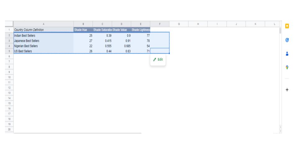
As I am trying to learn R more, I decided to process the same dataset in R, and figure out how to duplicate the same things I did in Google Sheets. I was able to group data (countries) together and used the following code to get the median of each individual column:

pivot_table_mean<-shades %>%
group_by(country_name) %>%
dplyr::summarise(hue_median=median(Hue), saturation_mean=mean(Saturation), value_mean=mean(Value), lightness_mean=mean(Lightness))

It created the following:

As can be seen, the "US Best Sellers" row is practically empty, and the value that is included is way off from the median I got when I did this using Google Sheets. (Note: I just went back and looked at my dataset: some columns in the US Best Sellers section DOES have na, meaning there is a bunch of info missing. However, some of the US Best Sellers information IS filled in. I'm thinking R is throwing everything out because it doesn't know what to do with the data that says na. Is there a way to remove the na's? OR a way to convert the na's to zero (0) AND, if so, will that affect the calculation results?)

As for the other variables: Some are close but not exact, and some are just plain "off". I've posted below the values from Google Sheets for comparison:

Any feedback is greatly appreciated as always.

I cannot read the image of your R results but I will take your word for it that the results differ. Can post a subset of your data that shows the problem? Running

dput(head(shades,50))

will give you output that you can post here and will allow others to use your data. Place a line with three back ticks before and after the posted output, like this:
```
output of dput
```
To deal with NA values, you can set the na.rm argument of median to TRUE

summarise(hue_median=median(Hue, na.rm = TRUE), ...
1 Like

We need a FAQ: How to do a minimal reproducible example ( reprex ) for beginners

The code you have supplied is good but would be useful to see all the code and to see some sample data. A handy way to supply some sample data is the dput() function. In the case of a large dataset something like dput(head(mydata, 100)) should supply the data we need.

One thing I did notice is that you are using group_by() and then dplyr::summarise. group_by is in the *dyplyr pagkage as is summarise. Have you loaded dplyer using a library(dplyr) command?

Yes, I installed and loaded dplyr prior to running the code.
To your first point about using reprex: When I first joined this community, there was an introduction that included information about using reprex (for beginners). I've posted several questions to the community since then and I have to confess that it is I that got lazy and forgot all about reprex. I was hoping the bits of information I was providing would be enough to get some valuable feedback. Going forward, however, I will try to adhere to the guidelines and use (first learn to use) reprex so that it is easier on anyone trying to help me. Thanks for the reminder and I apologize for not doing what I should have been doing.

dput(head(shades,50))
structure(list(brand = c("Maybelline", "Maybelline", "Maybelline", 
"Maybelline", "Maybelline", "Maybelline", "Maybelline", "Maybelline", 
"Maybelline", "Maybelline", "bareMinerals", "bareMinerals", "bareMinerals", 
"bareMinerals", "bareMinerals", "bareMinerals", "bareMinerals", 
"bareMinerals", "bareMinerals", "bareMinerals"), brand_short = c("mb", 
"mb", "mb", "mb", "mb", "mb", "mb", "mb", "mb", "mb", "mb", "mb", 
"mb", "mb", "mb", "mb", "mb", "mb", "bm", "bm", "bm", "bm", "bm", 
"bm", "bm", "bm", "bm", "bm"), product = c("Fit Me", "Fit Me", 
"Fit Me", "Fit Me", "Fit Me", "Fit Me", "Fit Me", "Fit Me", "Fit Me", 
"Fit Me", "Fit Me", "Fit Me", "barePRO", "barePRO", "barePRO", 
"barePRO", "barePRO", "barePRO", "barePRO", "barePRO", "barePRO", 
"barePRO"), product_short = c("fmf", "fmf", "fmf", "fmf", "fmf", 
"fmf", "fmf", "fmf", "fmf", "fmf", "fmf", "fmf", "fmf", "fmf", 
"fmf", "fmf", "fmf", "fmf", "fmf", "fmf", "fmf", "fmf", "pro", 
"pro", "pro", "pro", "pro", "pro", "pro", "pro", "pro", "pro"
), hex = c("f3cfb3", "ffe3c2", "ffe0cd", "ffd3be", "bd9584", 
"eabda6", "fbd2ad", "e2b597", "e4b38e", "b2856f", "e8ba8c", "f3b584", 
"f0b996", "e3b082", "eab181", "9d7359", "e2aa7b", "d99358", "9c744f", 
"b18b65", "84583f", "7d5631", "c07746", "643c27", "edcfb9", "e1bba7", 
"c1a07e", "d09e7c", "c7967d", "c09578", "9d6f48", "a86d40", "7f5c3b", 
"735642", "6b5041", "7d5c4d", "5c4433", "5e3a23", "5e4638", "3f2018", 
"edceb2", "f0cba1", "ebc99c", "e6bc94", "dcb79a", "eac8a3", "e9c89e", 
"d4ad8a", "cfa786", "d8b08c"), Hue = c(26, 32, 23, 19, 18, 20, 
28, 24, 26, 20, 30, 26, 23, 28, 27, 23, 27, 27, 29, 30, 22, 29, 
24, 21, 25, 21, 30, 24, 20, 24, 28, 26, 29, 24, 21, 19, 25, 23, 
22, 12, 28, 32, 34, 29, 26, 31, 34, 28, 27, 28), Saturation = c(0.26, 
0.24, 0.2, 0.25, 0.3, 0.29, 0.31, 0.33, 0.38, 0.38, 0.4, 0.46, 
0.37, 0.43, 0.45, 0.43, 0.46, 0.59, 0.49, 0.43, 0.52, 0.61, 0.64, 
0.61, 0.22, 0.26, 0.35, 0.4, 0.37, 0.38, 0.54, 0.62, 0.54, 0.43, 
0.39, 0.38, 0.45, 0.63, 0.4, 0.62, 0.25, 0.33, 0.34, 0.36, 0.3, 
0.3, 0.32, 0.35, 0.35, 0.35), Value = c(0.95, 1, 1, 1, 0.74, 
0.92, 0.98, 0.89, 0.89, 0.7, 0.91, 0.95, 0.94, 0.89, 0.92, 0.62, 
0.89, 0.85, 0.61, 0.69, 0.52, 0.49, 0.75, 0.39, 0.93, 0.88, 0.76, 
0.82, 0.78, 0.75, 0.62, 0.66, 0.5, 0.45, 0.42, 0.49, 0.36, 0.37, 
0.37, 0.25, 0.93, 0.94, 0.92, 0.9, 0.86, 0.92, 0.91, 0.83, 0.81, 
0.85), Lightness = c(86, 92, 91, 88, 65, 80, 87, 77, 77, 60, 
79, 79, 80, 76, 77, 52, 74, 67, 52, 61, 42, 40, 57, 30, 85, 79, 
68, 69, 66, 65, 51, 52, 42, 39, 37, 42, 31, 28, 32, 16, 85, 84, 
83, 79, 77, 83, 83, 74, 72, 75), group = c(2, 2, 2, 2, 2, 2, 
2, 2, 2, 2, 2, 2, 2, 2, 2, 2, 2, 2, 2, 2, 2, 2, 2, 2, 2, 2, 2, 
2, 2, 2, 2, 2, 2, 2, 2, 2, 2, 2, 2, 2, 2, 2, 2, 2, 2, 2, 2, 2, 
2, 2), country_name = c("US_Best_sellers", "US_Best_sellers", 
"US_Best_sellers", "US_Best_sellers", "US_Best_sellers", "US_Best_sellers", 
"US_Best_sellers", "US_Best_sellers", "US_Best_sellers", "US_Best_sellers"
)), row.names = c(NA, -50L), class = c("tbl_df", "tbl", "data.frame"
))
> 

I changed the summarise code and was able to remove the na's per your instructions. Thanks. That was a lot simpler than I thought it was going to be.

Screenshots are unhelpful. Please use a reprex.

As far as the general question of why

recall that R was invented, and has been extended and maintained, for use by statisticians for statisticians over a period 10 years longer than the existence of Google, beginning with the language S from Bell Labs in 1988. You've identified the source of the disconnect

median has an default argument of na.rm = FALSE because calculations involving NA evaluate to NA.

NA + 1
#> [1] NA

NA is not equivalent to 0 and shouldn't be treated as if it were.

Very good. Thank you.

When in doubt, it is safer to trust R assuming no errors in the code. Spreadsheets are cobbled together by computer programmers and they can give some peculiar and even nasty results sometimes.
curious.math.table.pdf (127.5 KB)

2 Likes

This topic was automatically closed 7 days after the last reply. New replies are no longer allowed.

If you have a query related to it or one of the replies, start a new topic and refer back with a link.