Im try to make this map, but when put the shape of the country but dont fall in the exactly position. I need that the layer fall in the exactly position. Is possible this?
My guess is it won't either. The boundaries look displaced overall. @M_AcostaCH you might have a problem with the CRSs. Check the crs of your basemap and data to make sure it's the same. I think you can do that with st_crs() from the sf package. If they are not the same, read up on st_transform().
Please don't answer twice with the same text. I thought something was wrong with the notification system of this discourse. I tried with NaturalEarth data, but the problem seems to persist.
This seems a bit cumbersome, but it's a starter. I hope someone drops by and improves on this solution, or, well, half of a solution.
For the region boundaries in Macedonia, you will need to look at the data table and try to come up with a better subsetting, but this is a good start.
---
title: "Adm 1 Poly Makedonia"
author: "M_AcostaCH"
date: "`r Sys.Date()`"
thread: https://forum.posit.co/t/how-put-the-shape-in-the-exactly-position-of-a-country/163639
output: html_document
runtime: shiny
---
```{r}
library(leaflet)
library(osmdata)
library(tidyverse)
library(ggmap)
# trying a working example with OSM data and stamen background map,
# because ggmap cannot get OSM tiles for some reason
# get the bbox. this looks ok
mkd_bb <- getbb("Macedonia", featuretype = "country")
# query overpass api. ok.
mkd_bb %>% opq()
# get the hospitals in Macedonia. ok so far
makedonia_hospitals <- mkd_bb %>%
opq() %>%
add_osm_feature(key = "amenity", value = "hospital") %>%
osmdata_sf()
makedonia_hospitals
# extract the hospital polygons. still ok.
mypoly <- makedonia_hospitals$osm_polygons
# plot without map background
ggplot() +
geom_sf(data = makedonia_hospitals$osm_polygons)
# get the map background
mkmap <- get_map(mkd_bb, source = "stamen", maptype = "toner-hybrid")
ggmap(mkmap) +
geom_sf(
data = mypoly,
inherit.aes = FALSE,
colour = "#125421",
fill = "#329832",
alpha = .5,
size = 1
) +
labs(x = "", y = "")
# looks gorgeous! Placement is just fine
leaflet() %>% addTiles() %>% addPolygons(data = mypoly)
# now to something completely different
# let's look at the available features. "boundary" is one of them
available_features()
# what tags are in boundary?
available_tags("boundary")
# this follows the exact same structure
# DO NOT RUN THIS, IT WILL DOWNLOAD 3.5 GIGABYTES OF DATA
makedonia_boundaries <- mkd_bb %>%
opq() %>%
add_osm_feature(key = "boundary", value = "administrative") %>%
osmdata_sf()
# this tries to limit the amount of downloaded data
# it still downloads over 800 MB of data, which is unnecessary
# For Northern Macedonia:
# admin_level=2 is supposedly the right admin level for the country
# admin_level=4 are regions and
# admin_level=7 are municipalities
adm <- mkd_bb %>%
opq() %>%
add_osm_feature(key = "boundary", value = "administrative") %>%
add_osm_feature(key = "admin_level",value = "4") %>%
osmdata_sf()
# out <- osmdata_sf(adm)
adm_poly <- adm$osm_polygons
adm_points <- adm$osm_points
adm_lines <- adm$osm_lines
# although the bbox is the same as above, this is weird
ggplot() +
geom_sf(data = adm_poly)
# and here we can see why
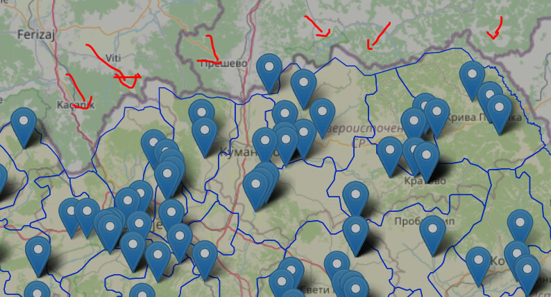
leaflet() %>% addTiles() %>% addPolygons(data = adm_poly)
# this is better
leaflet() %>% addTiles() %>% addPolylines(data = adm_lines)
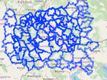
# subset the rows to just get Macedonia borders
# this explores how to filter the lines by two different columns with
# a colon character (:) in them, which is not trivial. One would expect
# an " around the column names, but instead, you need to use backticks, `.
lkj <- subset(adm_lines, `left:country` == "North Macedonia" | `right:country` == "North Macedonia")
# display in map
leaflet() %>% addTiles() %>% addPolylines(data = lkj)
This is more than enough explanation, I appreciate the time you spent for this.
I will review the code to understand it very well and try to modify it to get the political division of MKD.
# If I undestand well, im modify with 7 for municipalities, but map show more than only MKD.
adm <- mkd_bb %>%
  opq() %>%
  add_osm_feature(key = "boundary", value = "administrative") %>%
  add_osm_feature(key = "admin_level",value = "7") %>%
  osmdata_sf()
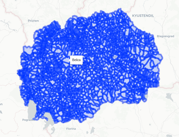
What it does is that it downloads a geojson of all European LAU units, filters the ones in Macedonia and displays them in a leaflet call.
The GISCO data are in WGS84 CRS, which is well compatible with Leaflet. The resolution is one to a million, which quite fine level of detail (and it shows in the size of downloaded file; but you need to download it only once).
Should you require another level of admin detail - say NUTS - there are calls in {giscoR} package to get those.