I don't know how to upload the shapefile, so the data, code and figure are shown below. Due to the large volume of the DFgrid file, I only included part of the dataset, but the dataframe structure is the same. The DFgrid covers whole shapefile border, but some grids are even outside of the border. I can only draw the two figures separately. How to crop the DFgrid file to the shapefile border, so that all grids are inside of the border and have perfect curves at the verge? I would really appreciate your help.
######################### example file
library(ggplot2)

DFgrid= data.frame(
  lon=c(59.25, 59.75, 60.25, 60.75, 61.25, 61.75, 57.25, 57.75, 58.25, 58.75, 59.25, 59.75, 60.25, 60.75, 61.25, 61.75, 62.25, 57.25, 57.75, 58.25, 58.75, 59.25, 59.75, 60.25, 60.75, 61.25, 61.75, 62.25, 62.75, 53.25),
  lat=c(25.25, 25.25, 25.25, 25.25, 25.25, 25.25, 25.75, 25.75, 25.75, 25.75, 25.75, 25.75, 25.75, 25.75, 25.75, 25.75, 25.75, 26.25, 26.25, 26.25, 26.25, 26.25, 26.25, 26.25, 26.25, 26.25, 26.25, 26.25, 26.25, 26.75),
  value= rnorm(30)
)

my_year <- theme_bw() + theme(panel.ontop=TRUE, panel.background=element_blank())
my_fill <- scale_fill_distiller('',palette='Spectral',
                                breaks = c(-2,0,2))

fig = ggplot(DFgrid, aes(y=lat, x=lon, fill=value)) + geom_tile() + my_year + my_fill+
  coord_quickmap(xlim=c(44.05, 63.35), ylim=c(25.05, 39.75))+
  borders('world', xlim=c(44.05, 63.35), ylim=c(25.05, 39.75), colour='black')+
  xlab('Longitude (°E)')+ ylab('Latitude (°N)')+
  theme(panel.grid=element_blank(),
        panel.border = element_rect(colour = "black", fill=NA,size=.7))
print(fig)

install.packages("maptools",repos="http://cran.us.r-project.org")
> library(maptools)
> library(rgdal)
> library(raster)
> setwd('C:/Users/Acer/Desktop/border_shape')
> list.files()
[1] "border.CPG" "border.dbf" "border.prj" "border.shp" "border.shp.xml"
[6] "border.shx"
> data.shape<-readOGR(dsn=".",layer="border")
OGR data source with driver: ESRI Shapefile
Source: "C:\Users\Acer\Desktop\border_shape", layer: "border"
with 1 features
It has 70 fields
Integer64 fields read as strings: ID_0 OBJECTID_1
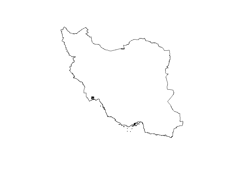
> plot(data.shape)
> class(data.shape) # Describes the type of vector data stored in the object.
[1] "SpatialPolygonsDataFrame"
attr(,"package")
[1] "sp"
> length(data.shape) # How many features are in this spatial object?
[1] 1
> extent(data.shape) # The spatial extent (geographic area covered by) features in the object.
class : Extent
xmin : 44.04726
xmax : 63.31746
ymin : 25.05875
ymax : 39.77722
> crs(data.shape) # coordinate reference system
CRS arguments:
+proj=longlat +datum=WGS84 +no_defs +ellps=WGS84 +towgs84=0,0,0
Plot it
> data.shape = readOGR(dsn='C:/Users/Acer/Desktop/border_shape/.',layer='border')
OGR data source with driver: ESRI Shapefile
Source: "C:\Users\Acer\Desktop\border_shape", layer: "border"
with 1 features
It has 70 fields
Integer64 fields read as strings: ID_0 OBJECTID_1
> plot(data.shape)