I have 32 months of data, and I'm trying out different models for testing the forecasting of cumulative monthly unit transitions to dead state "X" as a percentage of the total population of units at time 0 for months 13-32, by training from data for months 1-12. Note that the curve is the inverse of exponential decay, it's a logarithmic curve that climbs up and can never exceed 100% and can only climb up or flatten out; it can't curl down over time since the dead never return. I then compare the forecasts with the actual data for months 13-32. Not all beginning units die off, only a portion. I understand that 12 months of data for model training isn't much and that forecasting for 20 months from those 12 months should result in a wide distribution of outcomes, those are the real-world limitations I usually grapple with. I'm working through examples in Hyndman, R.J., & Athanasopoulos, G. (2021) Forecasting: principles and practice , 3rd edition, OTexts: Melbourne, Australia. Forecasting: Principles and Practice (3rd ed) with this data.
When I run the example in the book from section 5.5 Distributional forecasts and prediction intervals, Prediction intervals from bootstrapped residuals, Figure 5.15, adapted to my data (my data and code posted at the bottom), I get the simulation paths illustrated below (the heavy black line represents the actual data for those theoretical forecast months 13-32):
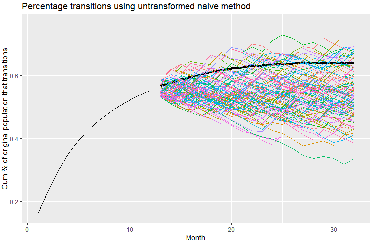
My question is, is there any type of transformation or type of model suited for a logarithmic function curve like this, where no cumulative forecast or distribution thereof can be less than the prior period value, and no cumulative forecast or distribution can exceed 100%? Or, alternatively, should I modify the data so it is not cumulative? Even so, if it's not cumulative, I'll have the same constraint that the total of pre-forecast values and forecast values can never exceed 100%. I've reviewed section ** 13.3 Ensuring forecasts stay within limits**, Forecasts constrained to an interval of the book where scaled logit transformations are introduced, but it addresses interval constraints, but not the sort of cumulative interval constraints I'm dealing with.
Here's my data and code:
library(dplyr)
library(fabletools)
library(fable)
library(feasts)
library(ggplot2)
library(tidyr)
library(tsibble)

DF <- data.frame(
  Month =c(1:32),
  rateCumX=c(
    0.1623159,0.23137659,0.29942238,0.35294557,0.39603576,0.42849893,0.45752922,0.48252959,
    0.50369408,0.52248541,0.53859013,0.55262019,0.56639651,0.57797878,0.58750131,0.59563576,
    0.60380006,0.61141211,0.61706891,0.62215854,0.62606905,0.62966611,0.63217361,0.63448708,
    0.63647219,0.63760653,0.63863640,0.63930805,0.63956178,0.63969611,0.63977074,0.63977074
  )
) %>%
  as_tsibble(index = Month)

fit_bstrp <- DF[1:12,] %>%
  model(NAIVE(rateCumX))
sim <- fit_bstrp %>% generate(h = 20, times = 100, bootstrap = TRUE)
DF[1:12,] %>%
  ggplot(aes(x = Month)) +
  autolayer(
    filter_index(DF, 13 ~ .), # 13th + month historical data
    colour = "black", size = 1.5) +
  geom_line(aes(y = rateCumX)) +
  geom_line(aes(y = .sim, colour = as.factor(.rep)),
            data = sim) +
  labs(title="Percentage transitions using untransformed naive method",
       y="Cum % of original population that transitions") +
  guides(colour = "none")
Referred here by Forecasting: Principles and Practice, by Rob J Hyndman and George Athanasopoulos