How to make a dataframe, containing the column of hours and the following column the counts

[MathieuVandamme]

Hi all

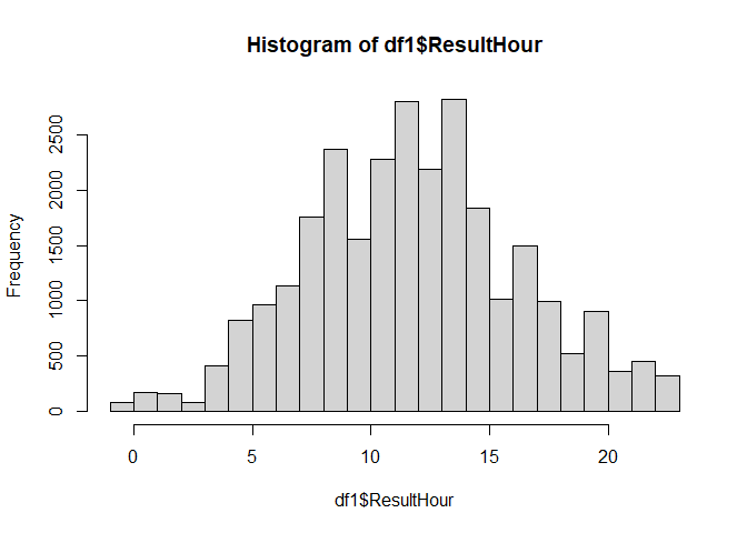
I have a dataset that contains testsamples and there result time. I want to visualize the amount of samples each hour and visualize it on a histogram. I use following code:

#Calculate the amount of Result-samples each hour:
df2 <- as.data.frame(hour(hms(df1_filtered$ResultTime)))
df_aggr_Result <- aggregate(df2, by=list(df2$`hour(hms(df1_filtered$ResultTime))`), FUN = length)

When a test is performed each hour, in the first column of the df_aggr_Result, the hours are going from 0 until 23 (like it supposed to be). I have a good histogram.

The problem occurs when eg. a test is done 7 times at 12h and 3 times at 18h. When I use the code above, I get a df_aggr_Result with only 2 rows (one row with 12h and the other with 18h), this results in a histogram with two "bars" and not the wanted 24 bars.
How can I code that the first column of the created dataframe counts from 0 untill 23 and add a 0 in the other column if it cannot be counted in the previous dataframe.

Here is a link to my intial CSV:
https://drive.google.com/file/d/14KSe_pdATXQJTZSJMOHKWExA_m7XCgJH/view?usp=sharing

Thanks in advance!

This is my total code:

knitr::opts_chunk$set(echo = TRUE)
install.packages(c("lubridate"),repos = "http://cran.us.r-project.org")
install.packages(c("dplyr"),repos = "http://cran.us.r-project.org")

knitr::include_graphics("https://weareofficemanagementmechelen.files.wordpress.com/2019/12/roche-logo.jpeg?w=400")

#First the exported file from the Infinity server needs to be in the correct folder and read in:
setwd("G:/My Drive/Traineeship Advanced Bachelor of Bioinformatics 2022/Internship 2022-2023/internship documents/")
server_data <- read.delim(file="PostCheckAnalysisRoche.txt", header = TRUE, na.strings=c(""," ","NA"))

#Create a subset of the data to remove/exclude the unnecessary columns:
subset_data_server <- server_data[,c(-5:-7,-9,-17,-25:-31)]
#Remove the rows with blank/NA values:
df1 <- na.omit(subset_data_server)
#The difference between the ResultTime and the FirstScanTime is the turn around time:
df1$TS_start <- paste(df1$FirstScanDate, df1$FirstScanTime)
df1$TS_end <- paste(df1$ResultDate, df1$ResultTime)
df1$TAT <- difftime(df1$TS_end,df1$TS_start,units = "mins")

library(lubridate)
library(dplyr)

selectInput(inputId='test', label='Test:',
            choices = df1$TestName)


df1_filtered <- df1[df1$TestName == "IGF",]

#Calculate the amount of Result-samples each hour:
df2 <- as.data.frame(hour(hms(df1_filtered$ResultTime)))
df_aggr_Result <- aggregate(df2, by=list(df2$`hour(hms(df1_filtered$ResultTime))`), FUN = length)
#Renaming
names(df_aggr_Result)[names(df_aggr_Result) == "Group.1"] <- "hour"
names(df_aggr_Result)[names(df_aggr_Result) == "hour(hms(df1_filtered$ResultTime))"] <- "amount of samples"

renderPlot({
  x <- as.numeric(df_aggr_Result$`amount of samples`)
  hist(x, breaks = 24,
          xlab = "Hours in a day",
          ylab = "Amount of samples"
            )
})

[FJCC]

Is this the sort of thing you are looking for?

server_data <- read.csv("~/R/Play/PostCheckAnalysis.csv",sep="\t",
                        na.strings = c(""," ","NA"))
subset_data_server <- server_data[,c(-5:-7,-9,-17,-25:-31)]
#Remove the rows with blank/NA values:
df1 <- na.omit(subset_data_server)
library(dplyr)
library(lubridate)
library(hms)
df1 <- df1 |> mutate(ResultHour=hour(as_hms(ResultTime)))
hist(df1$ResultHour,breaks = -1:23)

table(df1$ResultHour)
#> 
#>    0    1    2    3    4    5    6    7    8    9   10   11   12   13   14   15 
#>   79  169  165   85  412  820  960 1138 1758 2362 1559 2276 2795 2181 2812 1835 
#>   16   17   18   19   20   21   22   23 
#> 1015 1495  992  523  905  368  454  327

^{Created on 2022-10-13 with reprex v2.0.2}

[FJCC]

I realized I did not answer the part of your question about making a data frame with the counts.

df1_summary <- df1 |> group_by(ResultHour) |> 
   summarize(N=n())
df1_summary
# A tibble: 24 × 2
   ResultHour     N
        <int> <int>
 1          0    79
 2          1   169
 3          2   165
 4          3    85
 5          4   412
 6          5   820
 7          6   960
 8          7  1138
 9          8  1758
10          9  2362