I have 32 months of data, and I'm testing models for forecasting unit transitions to dead state "X" for months 13-32, by training from transitions data for months 1-12. I then compare the forecasts with the actual data for months 13-32. The data represents the unit migration of a beginning population into the dead state over 32 months. Not all beginning units die off, only a portion. I understand that 12 months of data for model training isn't much and that forecasting for 20 months from those 12 months should result in a wide distribution of outcomes. I'm using Hyndman, R.J., & Athanasopoulos, G. (2021) Forecasting: principles and practice , 3rd edition, OTexts: Melbourne, Australia. Forecasting: Principles and Practice (3rd ed) as a resource text.
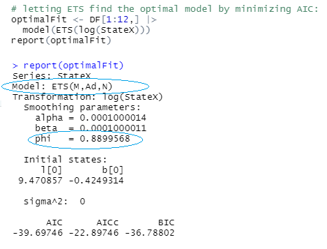
I'm working through section 8.2 Methods with trend, Figure 8.4, of the book with my data. The text states "We have set the damping parameter to a relatively low number (ϕ =0.90) to exaggerate the effect of damping for comparison" (value of phi parameter added to the trend component of the ETS function). I noticed that phi has a very large effect on fitting and resulting simulations.
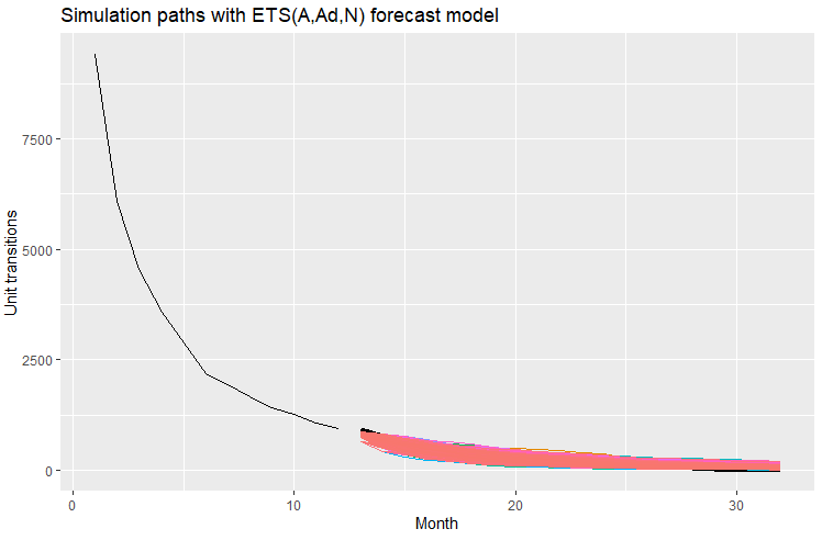
In the code at the bottom I optimize phi in order to most closely align model forecasts for forecast months 13-32 with actual data for those months 13-32. The idea being, when faced with similar data and exponential decay curve for months 1-12 (and lacking data for months beyond month 12), I would use the same phi value for forecasting beyond month 12. Is this a "statistically valid" approach? Robust? Or is this an example of rookie overfitting? Should I even be toying around with the phi parameter in model fitting?
When I run simulations with the optimized phi value of 0.9757943, I get the following results which I am pleased with from my experience with similar curves:
Code:
library(dplyr)
library(fabletools)
library(fable)
library(feasts)
library(ggplot2)
library(tidyr)
library(tsibble)

DF <- data.frame(
  Month =c(1:32),
  StateX=c(
    9416,6086,4559,3586,2887,2175,1945,1675,1418,1259,1079,940,923,776,638,545,547,510,379,
    341,262,241,168,155,133,76,69,45,17,9,5,0)
) %>%
  as_tsibble(index = Month)

myFunction <- function(x) {
  fit_A_Ad_N <- DF[1:12,] |> model(ETS(log(StateX) ~ error("A")+trend("Ad",phi = x)+season("N")))
  sim_A_Ad_N <- fit_A_Ad_N %>% generate(h = 20, times = 5000, bootstrap = TRUE)
  sim_A_Ad_N_DF <- as.data.frame(sim_A_Ad_N)
  agg_A_Ad_N <- sim_A_Ad_N_DF %>% group_by(.rep) %>% summarise(sum_FC = sum(.sim),.groups = 'drop')
  agg_A_Ad_N <- agg_A_Ad_N %>% as.data.frame()
  mean_A_Ad_N <- round(mean(agg_A_Ad_N[,"sum_FC"]),0)
  fc_actuals <- sum(as.data.frame(DF[13:32,2]))
  diff <- abs(mean_A_Ad_N - fc_actuals)
  return(diff)
}

f <- function(x) myFunction(x)
optimize(f, lower=0, upper=1)
Referred here by Forecasting: Principles and Practice, by Rob J Hyndman and George Athanasopoulos