Interpolation between variable dates

I have a large data frame that has random dates and 3 variables - h2, n2, and co2. A simplified version is below. I need to create a daily time series with the interpolated values of the variables - h2, n2 and co2 - for each day between the dates. The interpolation can be linear, or another form such as log-linear or cubic. The challenge I am facing is how to do the interpolation since the dates vary, and so will the number interpolated values for each variable. Any suggestions on how to interpolate variables between varying dates would be greatly appreciated.

Thanks in advance.

df <- data.frame("date"=c("20191102", "20191103", "20191201", "20200114", "20200201",  "20200303"),
                   "h2" = c(1.4,   2.5,  1.7,  0.2,  1.4,  0.1),
                   "n2"=c(0.4, 0.6, 0.75, 0.25, 0.9, 1.1),
                   "co2"=c(0.25, 0.40, 0.75, 0.8,  0.5, 0.6)) %>% 
  mutate(date=ymd(date))

There are 3 steps:

  • decide on a model
  • fit the model for each variable
  • predict new values

Model

You mention linear, that would be done with the function lm(). A generic way to make a smooth interpolation is loess(). Many other models do exist.

Fitting

In a base R approach, you can do the fitting like this:

mod_h2 <- lm(h2 ~ date, data = df)
mod_n2 <- loess(n2 ~ as.numeric(date), data = df)
mod_co2 <- lm(log(co2) ~ date, data = df)

You can use summary() to get details, and of course you need to check the assumptions (e.g. distribution of the residuals).

Prediction

Each model type has an associated predict() function, which takes the model, and a set of new x values, and predict the corresponding y values according to the model.

Reprex

So a complete example with some bad models and clumsy plotting:

library(dplyr)
#> 
#> Attaching package: 'dplyr'
#> The following objects are masked from 'package:stats':
#> 
#>     filter, lag
#> The following objects are masked from 'package:base':
#> 
#>     intersect, setdiff, setequal, union
library(tibble)
library(ggplot2)
library(lubridate)
#> 
#> Attaching package: 'lubridate'
#> The following objects are masked from 'package:base':
#> 
#>     date, intersect, setdiff, union

df <- data.frame("date"=c("20191102", "20191103", "20191201", "20200114", "20200201",  "20200303"),
                 "h2" = c(1.4,   2.5,  1.7,  0.2,  1.4,  0.1),
                 "n2"=c(0.4, 0.6, 0.75, 0.25, 0.9, 1.1),
                 "co2"=c(0.25, 0.40, 0.75, 0.8,  0.5, 0.6)) %>% 
  mutate(date=ymd(date))


mod_h2 <- lm(h2 ~ date, data = df)
mod_n2 <- loess(n2 ~ as.numeric(date), data = df)
mod_co2 <- lm(log(co2) ~ date, data = df)


new_df <- data.frame(date = seq(from = as.Date("2019-11-01"),
                                to = as.Date("2020-03-04"),
                                by="day"))

new_df <- new_df %>%
  mutate(h2 = predict(mod_h2, newdata = new_df),
         n2 = predict(mod_n2, newdata = new_df),
         co2 = predict(mod_co2, newdata = new_df))

df_both <- add_column(df, type = "observed") %>%
  bind_rows(add_column(new_df, type = "predicted"))

p_h2 <- ggplot(df_both) +
  theme_classic() +
  geom_point(aes(x = date, y = h2, color = type, size = type)) +
  scale_size_discrete(range = c(1, .2))
#> Warning: Using size for a discrete variable is not advised.

p_n2 <- ggplot(df_both) +
  theme_classic() +
  geom_point(aes(x = date, y = n2, color = type, size = type)) +
  scale_size_discrete(range = c(1, .2))
#> Warning: Using size for a discrete variable is not advised.

p_co2 <- ggplot(df_both) +
  theme_classic() +
  geom_point(aes(x = date, y = co2, color = type, size = type)) +
  scale_size_discrete(range = c(1, .2))
#> Warning: Using size for a discrete variable is not advised.


patchwork::wrap_plots(p_h2, p_n2, p_co2)
#> Warning: Removed 2 rows containing missing values (geom_point).

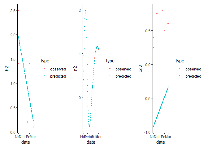
Created on 2023-01-05 by the reprex package (v2.0.1)

I further adapted this proposal by performing it over pairs of the observed data points; this results in a piecewise linear regression.

library(tidyverse)
library(lubridate)

df <- data.frame("date"=c("20191102", "20191103", "20191201", "20200114", "20200201",  "20200303"),
                 "h2" = c(1.4,   2.5,  1.7,  0.2,  1.4,  0.1),
                 "n2"=c(0.4, 0.6, 0.75, 0.25, 0.9, 1.1),
                 "co2"=c(0.25, 0.40, 0.75, 0.8,  0.5, 0.6)) %>% 
  mutate(date=ymd(date),
         rn=row_number())

(df_pairs <- map2(seq_len(nrow(df) - 1),
     1 + seq_len(nrow(df) - 1),
     ~df[c(.x,.y),]
))

(model_list <- map(df_pairs,
                  ~lm(h2~date,data=.x)))

(df_pairs_info <- map(df_pairs,
                     ~range(.x$date)) |> enframe(name="model_num",
                                                 value="date_range"))


(new_df <- data.frame(date = seq(from = min(df$date),
                                to = as.Date("2020-03-04"),
                                by="day")) |> rowwise() |> 
      mutate(list_of_possible = list(map_lgl(df_pairs_info$date_range,
                                             ~between(date,.x[1],.x[2]))),
             wpos  = list(which(list_of_possible)),
             wpos_clean = if_else(identical(wpos,integer(0)),list(length(model_list)),
                                  list(wpos)),
  model_to_use =  min(wpos_clean)) |> ungroup())

new_df <- new_df |> select(date,model_to_use) |> split(~model_to_use)


new_df_with_preds <- imap_dfr(new_df,
                         ~mutate(.x,
                                 h2=predict(model_list[[as.integer(.y)]],
                                           newdata=cur_data())))

df_both <- add_column(df, type = "observed") %>%
  bind_rows(add_column(new_df_with_preds, type = "predicted"))

p_h2 <- ggplot(df_both) +
  theme_classic() +
  geom_point(aes(x = date, y = h2, color = type, size = type)) +
  scale_size_discrete(range = c(1, .2))

1 Like

That makes me think, in a base R format, there is a function approx() that pretty much does this:

plot(approx(df$date, df$h2, method = "linear"))
points(df$date, df$h2, col = 'red')

image

It might also be worth checking out splines:

plot(spline(df$date, df$h2, n = 50))
points(df$date, df$h2, col = 'red')
1 Like

Thank-you everyone for your feedback. I was not aware of the base R functionality.

This topic was automatically closed 21 days after the last reply. New replies are no longer allowed.

If you have a query related to it or one of the replies, start a new topic and refer back with a link.