Interpreting decision trees

[fcas80]

Hi. Here is some code for a simple decision tree:

library(rpart)
library(rpart.plot)
df <- data.frame(x=c(1, 2, 3, 3, 3), y=c(0, 0, 1, 0, 1))
model<-rpart(y ~ x, data = df, method="class", minbucket = 1, minsplit=1, xval=5)
summary(model)
rpart.plot(model)

Here is the output for the cp table:

CP nsplit rel error xerror      xstd

1 0.50 0 1.0 1 0.5477226
2 0.01 1 0.5 2 0.4472136

Here is the output for the tree:

1. Is it possible to derive the numbers in the cp table? Do I need the results of each cross-validation?
2. Why does the top node contain 40% for 0? Shouldn't it be 60%?
3. Why does the bottom left leaf contain 0% for 0? Shouldn't it be 100%?

[FJCC]

The labeling of the plot, from top to bottom is

1. The most common element in the node.
2. The probability of an element being in the "second class", i.e. 1 in your data. There are no 1's in the bottom left leaf and in the right leaf, 2 of the 3 elements are 1.
3. 40% of the total population is in the bottom left leaf and 60% are in the right leaf.

I don't know how to generate the CP table.

[technocrat]

The cp table components can be extracted from the o object following

library(rpart)
library(rpart.plot)
df_ <- data.frame(x=c(1, 2, 3, 3, 3), y=c(0, 0, 1, 0, 1))
model<-rpart(y ~ x, data = df_, method="class", minbucket = 1, minsplit=1, xval=5)
(o <- summary(model)) |> str()
#> Call:
#> rpart(formula = y ~ x, data = df_, method = "class", minbucket = 1, 
#>     minsplit = 1, xval = 5)
#>   n= 5 
#> 
#>     CP nsplit rel error xerror      xstd
#> 1 0.50      0       1.0      1 0.5477226
#> 2 0.01      1       0.5      2 0.4472136
#> 
#> Variable importance
#>   x 
#> 100 
#> 
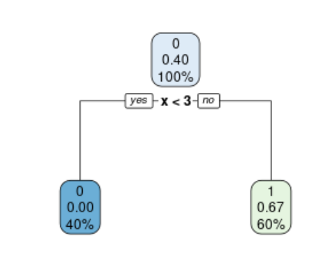
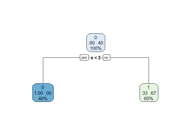
#> Node number 1: 5 observations,    complexity param=0.5
#>   predicted class=0  expected loss=0.4  P(node) =1
#>     class counts:     3     2
#>    probabilities: 0.600 0.400 
#>   left son=2 (2 obs) right son=3 (3 obs)
#>   Primary splits:
#>       x < 2.5 to the left,  improve=1.066667, (0 missing)
#> 
#> Node number 2: 2 observations
#>   predicted class=0  expected loss=0  P(node) =0.4
#>     class counts:     2     0
#>    probabilities: 1.000 0.000 
#> 
#> Node number 3: 3 observations
#>   predicted class=1  expected loss=0.3333333  P(node) =0.6
#>     class counts:     1     2
#>    probabilities: 0.333 0.667 
#> 
#> List of 14
#>  $ frame              :'data.frame': 3 obs. of  9 variables:
#>   ..$ var       : chr [1:3] "x" "<leaf>" "<leaf>"
#>   ..$ n         : int [1:3] 5 2 3
#>   ..$ wt        : num [1:3] 5 2 3
#>   ..$ dev       : num [1:3] 2 0 1
#>   ..$ yval      : num [1:3] 1 1 2
#>   ..$ complexity: num [1:3] 0.5 0.01 0.01
#>   ..$ ncompete  : int [1:3] 0 0 0
#>   ..$ nsurrogate: int [1:3] 0 0 0
#>   ..$ yval2     : num [1:3, 1:6] 1 1 2 3 2 1 2 0 2 0.6 ...
#>   .. ..- attr(*, "dimnames")=List of 2
#>   .. .. ..$ : NULL
#>   .. .. ..$ : chr [1:6] "" "" "" "" ...
#>  $ where              : Named int [1:5] 2 2 3 3 3
#>   ..- attr(*, "names")= chr [1:5] "1" "2" "3" "4" ...
#>  $ call               : language rpart(formula = y ~ x, data = df_, method = "class", minbucket = 1, minsplit = 1,      xval = 5)
#>  $ terms              :Classes 'terms', 'formula'  language y ~ x
#>   .. ..- attr(*, "variables")= language list(y, x)
#>   .. ..- attr(*, "factors")= int [1:2, 1] 0 1
#>   .. .. ..- attr(*, "dimnames")=List of 2
#>   .. .. .. ..$ : chr [1:2] "y" "x"
#>   .. .. .. ..$ : chr "x"
#>   .. ..- attr(*, "term.labels")= chr "x"
#>   .. ..- attr(*, "order")= int 1
#>   .. ..- attr(*, "intercept")= int 1
#>   .. ..- attr(*, "response")= int 1
#>   .. ..- attr(*, ".Environment")=<environment: R_GlobalEnv> 
#>   .. ..- attr(*, "predvars")= language list(y, x)
#>   .. ..- attr(*, "dataClasses")= Named chr [1:2] "numeric" "numeric"
#>   .. .. ..- attr(*, "names")= chr [1:2] "y" "x"
#>  $ cptable            : num [1:2, 1:5] 0.5 0.01 0 1 1 ...
#>   ..- attr(*, "dimnames")=List of 2
#>   .. ..$ : chr [1:2] "1" "2"
#>   .. ..$ : chr [1:5] "CP" "nsplit" "rel error" "xerror" ...
#>  $ method             : chr "class"
#>  $ parms              :List of 3
#>   ..$ prior: num [1:2(1d)] 0.6 0.4
#>   .. ..- attr(*, "dimnames")=List of 1
#>   .. .. ..$ : chr [1:2] "1" "2"
#>   ..$ loss : num [1:2, 1:2] 0 1 1 0
#>   ..$ split: num 1
#>  $ control            :List of 9
#>   ..$ minsplit      : num 1
#>   ..$ minbucket     : num 1
#>   ..$ cp            : num 0.01
#>   ..$ maxcompete    : int 4
#>   ..$ maxsurrogate  : int 5
#>   ..$ usesurrogate  : int 2
#>   ..$ surrogatestyle: int 0
#>   ..$ maxdepth      : int 30
#>   ..$ xval          : num 5
#>  $ functions          :List of 3
#>   ..$ summary:function (yval, dev, wt, ylevel, digits)  
#>   ..$ print  :function (yval, ylevel, digits, nsmall)  
#>   ..$ text   :function (yval, dev, wt, ylevel, digits, n, use.n)  
#>  $ numresp            : int 4
#>  $ splits             : num [1, 1:5] 5 -1 1.07 2.5 0
#>   ..- attr(*, "dimnames")=List of 2
#>   .. ..$ : chr "x"
#>   .. ..$ : chr [1:5] "count" "ncat" "improve" "index" ...
#>  $ variable.importance: Named num 1.07
#>   ..- attr(*, "names")= chr "x"
#>  $ y                  : int [1:5] 1 1 2 1 2
#>  $ ordered            : Named logi FALSE
#>   ..- attr(*, "names")= chr "x"
#>  - attr(*, "xlevels")= Named list()
#>  - attr(*, "ylevels")= chr [1:2] "0" "1"
#>  - attr(*, "class")= chr "rpart"

^{Created on 2023-03-09 with reprex v2.0.2}

[fcas80]

Thanks FJCC, but I'm still confused.

Each node has three numbers. The top number is the most common element. The bottom number is the percent of the population. Shouldn't the middle number be the proportion of the top number for the elements in that node? Are you saying the middle number is always the proportion of 1's? There's something counter-intuitive of that.

[FJCC]

What is displayed in the plot nodes is controlled by the extra argument and that defaults to 106 for a binary class model. The meaning of the 6 part of 106 is:

6 Class models: the probability of the second class only.

The 100 part of 106 is what causes the percentage of observations to be shown.
If I change the value of extra to 104, the nodes show the fraction of both levels, as in the second plot below.

library(rpart)
library(rpart.plot)
#> Warning: package 'rpart.plot' was built under R version 4.2.2
df <- data.frame(x=c(1, 2, 3, 3, 3), y=c(0, 0, 1, 0, 1))
model<-rpart(y ~ x, data = df, method="class", minbucket = 1, minsplit=1, xval=5)

rpart.plot(model, extra = 106)

rpart.plot(model, extra = 104)

^{Created on 2023-03-10 with reprex v2.0.2}

[fcas80]

FJCC, that makes sense, thank you.

I am still hoping someone can explain the cp table.

[FJCC]

I read about the cp table in the document linked below (starting at page 12) and I don't see any way to reproduce the cp table without running the cross validation. The key column is the cross validation error (xerror) and the information to derive that is not stored in the rpart.object, as far as I can see.

longintro.pdf