Llnear regression involving binary variables

[technocrat]

Rick@starz and I (Richard Careaga) invite discussion on when lm() should be avoided for binary values if at all? What alternative techniques should be considered?

• Continuous against continuous: both sides of the lm() formula are continuous variables
• Continuous against binary: left-hand side (LHS) continuous response with a binary predictor (right hand side RHS)
• Binary against continuous: A LHS binary response with a RHS continuous predictor
• Binary against binary: Both LHS and RHS are binary.

As a motivating example, mtcars includes four variables mpg, drat, vs and am

From help(mtcars)

mpg Miles/(US) gallon
drat Rear axle ratio
vs Engine (0 = V-shaped, 1 = straight)
am Transmission (0 = automatic, 1 = manual)

LHS continuous and RHS continuous

In the usual case of ordinary least squares linear regression both the LHS response variable and the RHS predictor variable are continuous

require(ggplot2)
#> Loading required package: ggplot2
mtcars |> ggplot(aes(drat,mpg)) +
  geom_point() +
  geom_smooth(method = "lm") +
  theme_minimal()
#> `geom_smooth()` using formula = 'y ~ x'

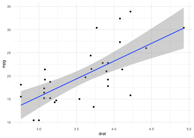
(fit <- lm(mpg ~ drat, data = mtcars))
#> 
#> Call:
#> lm(formula = mpg ~ drat, data = mtcars)
#> 
#> Coefficients:
#> (Intercept)         drat  
#>      -7.525        7.678
summary(fit)
#> 
#> Call:
#> lm(formula = mpg ~ drat, data = mtcars)
#> 
#> Residuals:
#>     Min      1Q  Median      3Q     Max 
#> -9.0775 -2.6803 -0.2095  2.2976  9.0225 
#> 
#> Coefficients:
#>             Estimate Std. Error t value Pr(>|t|)    
#> (Intercept)   -7.525      5.477  -1.374     0.18    
#> drat           7.678      1.507   5.096 1.78e-05 ***
#> ---
#> Signif. codes:  0 '***' 0.001 '**' 0.01 '*' 0.05 '.' 0.1 ' ' 1
#> 
#> Residual standard error: 4.485 on 30 degrees of freedom
#> Multiple R-squared:  0.464,  Adjusted R-squared:  0.4461 
#> F-statistic: 25.97 on 1 and 30 DF,  p-value: 1.776e-05
par(mfrow = c(2,2))
plot(fit)

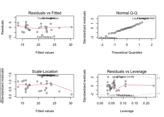
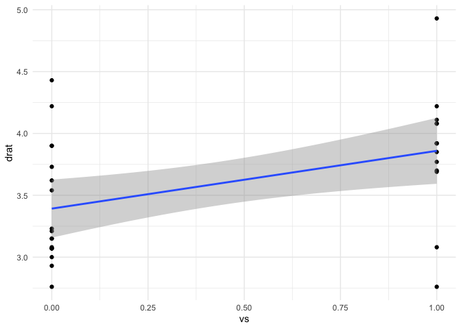
LHS continuous and RHS binary

require(ggplot2)
#> Loading required package: ggplot2
mtcars |> ggplot(aes(vs,drat)) +
  geom_point() +
  geom_smooth(method = "lm") +
  theme_minimal()
#> `geom_smooth()` using formula = 'y ~ x'

(fit2 <- lm(drat ~ vs, data = mtcars))
#> 
#> Call:
#> lm(formula = drat ~ vs, data = mtcars)
#> 
#> Coefficients:
#> (Intercept)           vs  
#>      3.3922       0.4671
summary(fit2)
#> 
#> Call:
#> lm(formula = drat ~ vs, data = mtcars)
#> 
#> Residuals:
#>      Min       1Q   Median       3Q      Max 
#> -1.09929 -0.31472 -0.04929  0.23351  1.07071 
#> 
#> Coefficients:
#>             Estimate Std. Error t value Pr(>|t|)    
#> (Intercept)   3.3922     0.1150  29.492   <2e-16 ***
#> vs            0.4671     0.1739   2.686   0.0117 *  
#> ---
#> Signif. codes:  0 '***' 0.001 '**' 0.01 '*' 0.05 '.' 0.1 ' ' 1
#> 
#> Residual standard error: 0.488 on 30 degrees of freedom
#> Multiple R-squared:  0.1938, Adjusted R-squared:  0.167 
#> F-statistic: 7.214 on 1 and 30 DF,  p-value: 0.01168
par(mfrow = c(2,2))
plot(fit2)

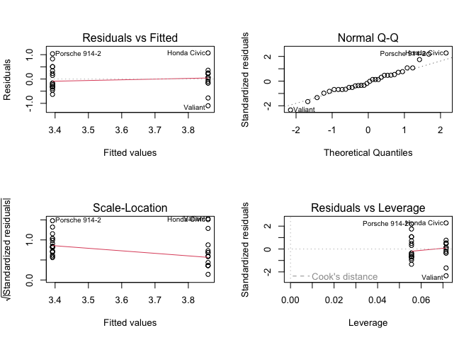
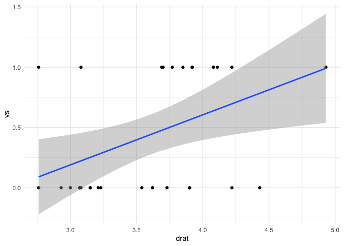
RHS binary and RHS continuous

require(ggplot2)
#> Loading required package: ggplot2
mtcars |> ggplot(aes(drat,vs)) +
  geom_point() +
  geom_smooth(method = "lm") +
  theme_minimal()
#> `geom_smooth()` using formula = 'y ~ x'

(fit3 <- lm(vs ~ drat, data = mtcars))
#> 
#> Call:
#> lm(formula = vs ~ drat, data = mtcars)
#> 
#> Coefficients:
#> (Intercept)         drat  
#>      -1.055        0.415
summary(fit3)
#> 
#> Call:
#> lm(formula = vs ~ drat, data = mtcars)
#> 
#> Residuals:
#>     Min      1Q  Median      3Q     Max 
#> -0.7834 -0.2791 -0.1754  0.4283  0.9097 
#> 
#> Coefficients:
#>             Estimate Std. Error t value Pr(>|t|)  
#> (Intercept)  -1.0552     0.5617  -1.879   0.0700 .
#> drat          0.4150     0.1545   2.686   0.0117 *
#> ---
#> Signif. codes:  0 '***' 0.001 '**' 0.01 '*' 0.05 '.' 0.1 ' ' 1
#> 
#> Residual standard error: 0.46 on 30 degrees of freedom
#> Multiple R-squared:  0.1938, Adjusted R-squared:  0.167 
#> F-statistic: 7.214 on 1 and 30 DF,  p-value: 0.01168
par(mfrow = c(2,2))
plot(fit3)

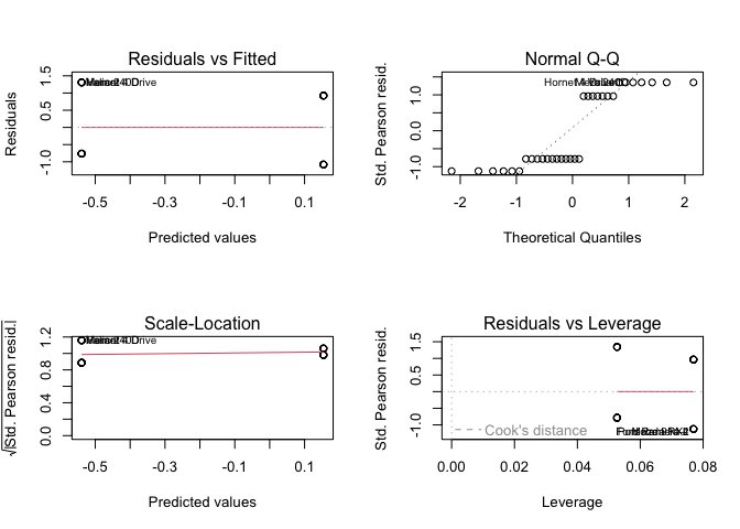
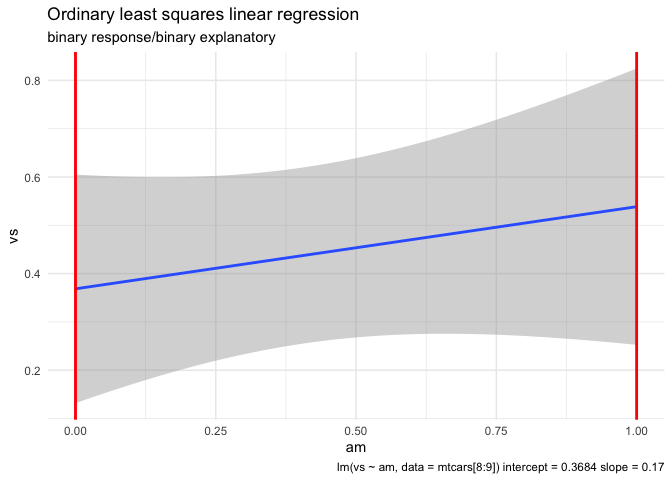
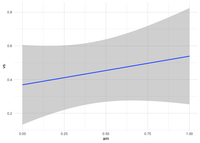
LHS binary and RHS binary

require(ggplot2)
#> Loading required package: ggplot2
mtcars |> ggplot(aes(am,vs)) +
  geom_point() +
  geom_smooth(method = "lm") +
  theme_minimal()
#> `geom_smooth()` using formula = 'y ~ x'

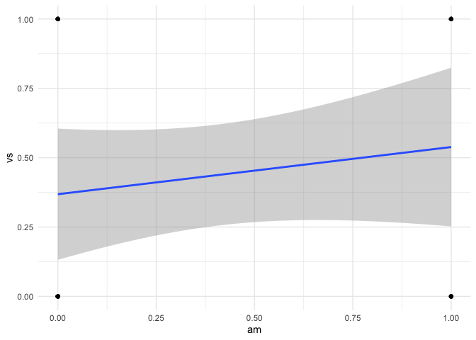
(fit4 <- lm(vs ~ am, data = mtcars))
#> 
#> Call:
#> lm(formula = vs ~ am, data = mtcars)
#> 
#> Coefficients:
#> (Intercept)           am  
#>      0.3684       0.1700
summary(fit4)
#> 
#> Call:
#> lm(formula = vs ~ am, data = mtcars)
#> 
#> Residuals:
#>     Min      1Q  Median      3Q     Max 
#> -0.5385 -0.3684 -0.3684  0.4615  0.6316 
#> 
#> Coefficients:
#>             Estimate Std. Error t value Pr(>|t|)   
#> (Intercept)   0.3684     0.1159   3.180  0.00341 **
#> am            0.1700     0.1818   0.935  0.35704   
#> ---
#> Signif. codes:  0 '***' 0.001 '**' 0.01 '*' 0.05 '.' 0.1 ' ' 1
#> 
#> Residual standard error: 0.505 on 30 degrees of freedom
#> Multiple R-squared:  0.02834,    Adjusted R-squared:  -0.004049 
#> F-statistic: 0.875 on 1 and 30 DF,  p-value: 0.357
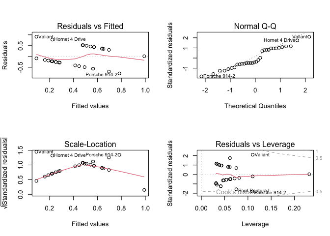
par(mfrow = c(2,2))
plot(fit4)

^{Created on 2023-04-09 with reprex v2.0.2}

[startz]

@technocrat, nicely laid out. Perhaps you could pick one and tell us what problems, if any, you have with the results.

[technocrat]

LHS continuous and RHS continuous is not problematic so long as the diagnostics get proper attention and overfitting is avoided.

LHS continuous and RHS binary had the awkward situation of a regression curve that has an intercept and slope for only the beginning and end, with nothing in between, as there is no Schrödinger’s binary provided for or a quantum regression methodology to go with it.

LHS binary and RHS continuous is an issue discussed recently here with one view being that it should never be used over logistic regression and the other that so long as R^2 is ignored ordinary least squares may be used.

LHS binary and R binary under logit regression

summary(fit5 <- glm(vs ~ am, data = mtcars, family = binomial(link = logit)))
#> 
#> Call:
#> glm(formula = vs ~ am, family = binomial(link = logit), data = mtcars)
#> 
#> Deviance Residuals: 
#>     Min       1Q   Median       3Q      Max  
#> -1.2435  -0.9587  -0.9587   1.1127   1.4132  
#> 
#> Coefficients:
#>             Estimate Std. Error z value Pr(>|z|)
#> (Intercept)  -0.5390     0.4756  -1.133    0.257
#> am            0.6931     0.7319   0.947    0.344
#> 
#> (Dispersion parameter for binomial family taken to be 1)
#> 
#>     Null deviance: 43.860  on 31  degrees of freedom
#> Residual deviance: 42.953  on 30  degrees of freedom
#> AIC: 46.953
#> 
#> Number of Fisher Scoring iterations: 4
par(mfrow = c(2,2))
plot(fit5)

appears to have the same diagnostic plot issues as the lm() example. Should different diagnostics be used? Is it simply the arbitrary selection of variables? Insufficient data? Are non-parametric required?

[startz]

This is a very good example. While there can certainly be important reasons to prefer one estimation method over another when there are binary variables, this example demonstrates that there is not a general argument against using a linear probability model.

@technocrat gives estimates from a linear probability model. When am==0, the probability of vs==1 is 0.3684. When am--1, the probability of vs==1 is .3684+.1700==0.5384.

@technocrat then gives estimates from a logit. Using the result that the prediction is exp(X\beta)/(1+exp(X\beta)) we get the estimates 0.3684 and 0.5384. Which are identical.

Just looking at the raw probabilities in the data,

library(tidyverse)
mtcars |> summarise(mean(vs), .by=am)
#>   am  mean(vs)
#> 1  1 0.5384615
#> 2  0 0.3684211

^{Created on 2023-04-10 with reprex v2.0.2}

we get exactly the same numbers.

So I think this illustrates that there is no general principle against using a lpm.

[technocrat]

The identical results for lm() and glm() that @startz notes raises something to think about: Does this result mean that the models are equally useful or does it mean that they are equally useless?

[startz]

@technocrat

Does this result mean that the models are equally useful or does it mean that they are equally useless?

Yes.

---

PS Note that they also exactly match the observed probabilities in the data, which suggests to me that they are about the best one can do.

[technocrat]

Both regression modes are less accurate than applying probabilities derived from simple contingency tables against unseen data.

library(DescTools)

mape <- function(x) MAPE(make_ct(lm(vs ~ am, data = mtcars)),ds[[x]])
smape <- function(x) SMAPE(make_ct(lm(vs ~ am, data = mtcars)),ds[[x]])
mse <- function(x) MSE(make_ct(lm(vs ~ am, data = mtcars)),ds[[x]])
rmse <- function(x) RMSE(make_ct(lm(vs ~ am, data = mtcars)),ds[[x]])
mape_self <- function(x) MAPE(self,ds[[x]])
smape_self <- function(x) SMAPE(self,ds[[x]])
mse_self <- function(x) MSE(self,ds[[x]])
rmse_self <- function(x) RMSE(self,ds[[x]])

make_ct <- function(x) {
  q1 = coef(x)[1]
  q2 = 1 - q1 
  q3 = q1 + coef(x)[2]
  q4 = 1 - q3
  ct = c(q1,q2,q3,q4)
  attributes(ct) = NULL
  ct = matrix(ct,nrow = 2)
  colnames(ct) = c("vs","am")
  return(ct)
}

# synthetic data
tiny_test <- data.frame(
  vs = sample(0:1,1e1,replace = TRUE),
  am = sample(0:1,1e1,replace = TRUE))
small_test <- data.frame(
  vs = sample(0:1,1e2,replace = TRUE),
  am = sample(0:1,1e2,replace = TRUE))
large_test <- data.frame(
  vs = sample(0:1,1e3,replace = TRUE),
  am = sample(0:1,1e3,replace = TRUE))
larger_test <- data.frame(
  vs = sample(0:1,1e4,replace = TRUE),
  am = sample(0:1,1e4,replace = TRUE))
huge_test <- data.frame(
  vs = sample(0:1,1e5,replace = TRUE),
  am = sample(0:1,1e5,replace = TRUE))
mega_test <- data.frame(
  vs = sample(0:1,1e6,replace = TRUE),
  am = sample(0:1,1e6,replace = TRUE))

# synthetic data as list of contingency tables
ds <- list(
  table(tiny_test)/nrow(tiny_test),
  table(small_test)/nrow(small_test),
  table(large_test)/nrow(large_test),
  table(larger_test)/nrow(larger_test),
  table(huge_test)/nrow(huge_test), 
  table(mega_test)/nrow(mega_test) 
)

# proportions table for mtcars[8:9]
(self <- table(mtcars[8:9])/nrow(mtcars))
#>    am
#> vs        0       1
#>   0 0.37500 0.18750
#>   1 0.21875 0.21875

(naive <- data.frame(
  dataset = c("tiny_1e1",
              "small_1e2","large_1e3",
              "larger_1e4","huge_1e5",
              "mega_1e6"),
  mape = sapply(1:6,mape_self),
  smape = sapply(1:6,smape_self),
  mse = sapply(1:6,mse_self),
  rmse = sapply(1:6,rmse_self)
))
#>      dataset      mape     smape         mse       rmse
#> 1   tiny_1e1 0.9166667 0.5614848 0.025371094 0.15928306
#> 2  small_1e2 0.3458130 0.3140000 0.010852344 0.10417458
#> 3  large_1e3 0.1458543 0.1470929 0.002475469 0.04975408
#> 4 larger_1e4 0.2419767 0.2310639 0.005030829 0.07092834
#> 5   huge_1e5 0.2501399 0.2382604 0.005387232 0.07339776
#> 6   mega_1e6 0.2493073 0.2375374 0.005351239 0.07315216

# proportions table for lm() fit

make_ct(lm(vs ~ am, data = mtcars))
#>             vs        am
#> [1,] 0.3684211 0.5384615
#> [2,] 0.6315789 0.4615385

# accuracy for ols regression

MAPE(lm(vs ~ am, data = mtcars))
#> [1] Inf
MSE(lm(vs ~ am, data = mtcars))
#> [1] 0.2391194
RMSE(lm(vs ~ am, data = mtcars))
#> [1] 0.4889984

# accuracy measures for synthetic data sets composed
# of sampling 0:1 in order of magnitude
# increments

(results <- data.frame(
  dataset = c("tiny_1e1",
              "small_1e2","large_1e3",
              "larger_1e4","huge_1e5",
              "mega_1e6"),
  mape = sapply(1:6,mape),
  smape = sapply(1:6,smape),
  mse = sapply(1:6,mse),
  rmse = sapply(1:6,rmse)
  ))
#>      dataset      mape     smape        mse      rmse
#> 1   tiny_1e1 1.2807018 0.7127454 0.06623826 0.2573679
#> 2  small_1e2 1.1000199 0.6623384 0.07362551 0.2713402
#> 3  large_1e3 1.0554349 0.6431717 0.07700932 0.2775055
#> 4 larger_1e4 1.0047927 0.6431688 0.07245760 0.2691795
#> 5   huge_1e5 0.9996751 0.6437874 0.07185494 0.2680577
#> 6   mega_1e6 1.0001569 0.6437165 0.07191563 0.2681709

cbind(naive[1],naive[2:5]-results[2:5])
#>      dataset       mape      smape         mse        rmse
#> 1   tiny_1e1 -0.3640351 -0.1512606 -0.04086717 -0.09808488
#> 2  small_1e2 -0.7542068 -0.3483384 -0.06277316 -0.16716562
#> 3  large_1e3 -0.9095806 -0.4960789 -0.07453385 -0.22775145
#> 4 larger_1e4 -0.7628160 -0.4121049 -0.06742677 -0.19825115
#> 5   huge_1e5 -0.7495351 -0.4055270 -0.06646771 -0.19465995
#> 6   mega_1e6 -0.7508496 -0.4061792 -0.06656439 -0.19501874

[startz]

I'm not following what you're doing here. Using the example data, both methods give identical results to using a contingency table.

[technocrat]

Sorry to be obscure, but I've found more convincing evidence anyway, and it's a good reminder of the importance of visualization.

library(ggplot2)
fit <- lm(vs ~ am, data = mtcars) 
fit |>
  ggplot(aes(am,vs)) +
    geom_smooth(method = "lm") +
    labs(title = "Ordinary least squares linear regression",
       subtitle = "binary response/binary explanatory",
       caption = paste(
         "lm(vs ~ am, data = mtcars[8:9]) intercept =",
        round(coef(fit)[1],4),
         "slope =",
        round(coef(fit)[2],4)
       )) +
  geom_vline(xintercept = 0, linewidth = 1, color = "red") +
  geom_vline(xintercept = 1, linewidth = 1, color = "red") +
    theme_minimal()
#> `geom_smooth()` using formula = 'y ~ x'

^{Created on 2023-04-12 with reprex v2.0.2}

Both vs and am can take on values of 1 and 0 in the closed interval [0,1] of the natural numbers. Neither can take on the value of any rational or irrational fraction, a negative value or a positive value in excess of one.

Using the slope of the regression line, there is no permitted value of am at which vs equals either one or zero. All that linear regression can tell us then is that the value of vs is undefined at am = 0 and am = 1.

[startz]

Cool visualization. I learned from it.

A linear probability model, or for that matter a logit, predicts the probability that the dependent variable equals 1.0 rather than directly predicting the dependent variable itself. So any predicted value in [0,1] is valid.

Of course, one important advantage of the logit is that it guarantees that predictions will be in [0,1]. The related problem with a linear probability model is that it may generate predictions outside [0,1], although that is not the case here. In fact, in the very simple case of a binary variable regressed on another binary variable, the linear probability model will never predict outside [0,1].

[startz]

Just used some of the lines from the ggplot() visualization in a graph I made today.

[technocrat]

lm()'s intercept taken as P(vs = 1 | am = 0) is 0.36842 and the addition of 1m()'s coefficient gives P(vs = 1 |am = 0) as 0.17004—in both cases the observed frequencies are 0.21875. Everything can be reduced to the following

(fit <- lm(vs ~ am, data = mtcars[8:9])) |>
ggplot2::ggplot(ggplot2::aes(am,vs)) +
  ggplot2::geom_smooth(method = "lm") +
  ggplot2::theme_minimal()
#> `geom_smooth()` using formula = 'y ~ x'

table(mtcars[8:9])
#>    am
#> vs   0  1
#>   0 12  6
#>   1  7  7
(tab <- table(mtcars[8:9])/sum(table(mtcars[8:9])))
#>    am
#> vs        0       1
#>   0 0.37500 0.18750
#>   1 0.21875 0.21875
fit$coefficients
#> (Intercept)          am 
#>   0.3684211   0.1700405
sum(fit$coefficients)
#> [1] 0.5384615
addmargins(tab)
#>      am
#> vs          0       1     Sum
#>   0   0.37500 0.18750 0.56250
#>   1   0.21875 0.21875 0.43750
#>   Sum 0.59375 0.40625 1.00000