Hi everyone,
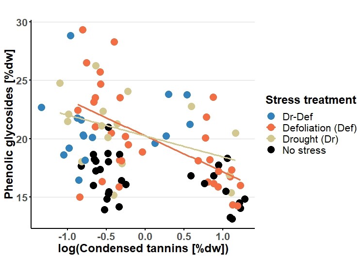
I would like to plot error bands around the orange and the yellowish plot lines whereas no error bands should be plotted for the blue and the black dots (see Fig).
How do I achive this? both the color of the "geom_smooth" and the "geom_fill" cannot be independently manipulated. I posted an example below in which I disabled the drawing of the error band (i.e. se=F in the geom_smooth command)
Thanks a lot for your help
Michael
data<-structure(list(CT_percent_dw = c(3.055555556, 3.409090909, 3.360215054,
3.315789474, 3.602362205, 3.086642599, 2.559726962, 2.232824427,
3.409090909, 2.978723404, 3.284883721, 3.016605166, 3.192041522,
2.952961672, 0.666666667, 1.810344828, 1.304347826, 1.781609195,
1.132075472, 1.349480969, 1.711956522, 0.517857143, 0.616438356,
0.510416667, 0.510638298, 0.610671937, 0.571428571, 0.802816901,
0.645104895, 0.718867925, 0.418478261, 0.696428571, 0.372093023,
0.742474916, 0.579150579, 0.615789474, 0.424914676, 0.349315068,
0.45112782, 0.416666667, 0.43772242, 2.819343066, 2.575757576,
2.984429066, 2.87109375, 2.142857143, 2.408759124, 1.8, 2.191901408,
2.293814433, 2.17472119, 2.405660377, 1.972318339, 3.036971831,
2.409747292, 2.572992701, 0.719557196, 0.622340426, 0.528169014,
0.625, 0.619791667, 0.436643836, 0.557761733, 0.430795848, 0.720430108,
0.446488294, 0.513422819, 0.469072165, 0.670648464, 0.559782609,
0.623239437, 0.776978417, 0.528169014, 0.711864407, 0.591796875,
0.734899329, 0.774368231, 0.525, 0.561776062, 0.734899329, 0.711956522,
0.963898917, 0.525, 0.439929329, 0.331578947, 0.366666667, 0.527777778,
0.796232877, 0.570588235, 0.262081784, 0.45959596, 0.448943662,
0.375, 0.505434783, 0.380681818), Pgpctsum = c(13.10100945, 14.03673316,
14.49033379, 14.20816207, 14.82049752, 14.31834663, 15.88320471,
16.26222056, 15.99855401, 16.7586737, 14.25929587, 15.36294444,
20.4937829, 16.90591139, 15.15631183, 22.7635716, 20.21575313,
21.22385497, 19.61140996, 23.80658212, 23.76776508, 18.21564315,
18.75050239, 18.66763459, 16.00376874, 14.83957532, 16.30774913,
19.49650719, 20.49798949, 18.15922748, 22.44657632, 21.26352884,
22.0857716, 17.86958824, 22.34934497, 20.0878363, 16.45076702,
18.61461888, 20.22716516, 21.77610898, 21.61290398, 15.47781773,
17.72589645, 13.24205241, 18.32590611, 16.14200976, 16.80843022,
16.82300431, 21.87117205, 18.1808839, 20.08058227, 23.5485354,
18.1125673, 17.30384798, 16.16080714, 17.21315326, 18.650118,
20.9817806, 18.07990634, 15.44913819, 18.02141379, 17.66843885,
17.37556129, 14.98621478, 23.52376447, 29.35898523, 23.13026266,
26.52283678, 28.29012736, 25.71698236, 15.2704095, 16.05241869,
17.23668338, 14.14301824, 13.91135314, 16.39329887, 20.18792759,
21.02312301, 24.68641607, 18.11268841, 15.88482023, 18.86816297,
23.52210358, 18.04458379, 24.7702106, 21.463626, 26.25516317,
24.04047496, 21.12506343, 22.69767598, 18.16931978, 20.33538331,
19.20997483, 20.1073092, 28.82528598), Category = c("CW", "CW",
"CW", "CW", "CW", "BeW", "BeW", "BeW", "BeW", "BeW", "BeW", "CD",
"CD", "CD", "CD", "CD", "BeD", "BeD", "BeD", "BeD", "BeD", "CW",
"CW", "CW", "CW", "CW", "BeW", "BeW", "BeW", "BeW", "BeW", "CD",
"CD", "CD", "CD", "CD", "BeD", "BeD", "BeD", "BeD", "BeD", "CW",
"CW", "CW", "CW", "CW", "CW", "CW", "BeW", "BeW", "BeW", "BeW",
"BeW", "BeW", "BeW", "BeW", "CW", "CW", "CW", "CW", "CW", "CW",
"CW", "BeW", "BeW", "BeW", "BeW", "BeW", "BeW", "BeW", "CW",
"CW", "CW", "CW", "CW", "CW", "BeW", "BeW", "BeW", "BeW", "BeW",
"BeW", "BeW", "CD", "CD", "CD", "CD", "CD", "CD", "BeD", "BeD",
"BeD", "BeD", "BeD", "BeD")), class = "data.frame", row.names = c(NA,
-95L))
ggplot(data, aes(x=log(CT_percent_dw),y=Pgpctsum, color=Category, linetype=Category)) +
geom_point(aes(fill=Category,color=Category),alpha=1, size=5, shape=21) +
geom_smooth(method="lm", alpha=0.4, linewidth=1.2,se=F, aes(fill=Category))+# group=1 necessary for drawing line
scale_fill_manual(values=c("#3182bd","#f46d43","#d3c88f","black"),labels=c("CW"="No stress","CD"="Drought (Dr)","BeW"="Defoliation (Def)","BeD"="Dr-Def"))+
scale_color_manual(values=c("#3182bd","#f46d43","#d3c88f","black"),labels=c("CW"="No stress","CD"="Drought (Dr)","BeW"="Defoliation (Def)","BeD"="Dr-Def"))+
scale_linetype_manual(values=c("blank","solid","solid","blank"),labels=c("CW"="No stress","CD"="Drought (Dr)","BeW"="Defoliation (Def)","BeD"="Dr-Def"))+
labs(title = "", y = "Phenolic glycosides [%dw]", x="log(Condensed tannins [%dw])")+
guides(fill=guide_legend(title="Stress treatment"))+
guides(color=guide_legend(title="Stress treatment"))+
guides(linetype=guide_legend(title="Stress treatment"))+
#Legend labels
theme(legend.position="right")+
#define theme
theme_classic() +
theme(axis.text=element_text(face="bold",size=16),
axis.title = element_text(color="black",face="bold",size=18),
axis.line = element_line(colour = 'black', size = 1),
axis.ticks = element_line(colour = "black", size = 1),
legend.text=element_text(size=16),
legend.title=element_text(size=18, face="bold"),
panel.grid.major.y = element_line(colour = "grey85",size = .5),
plot.title = element_text(color="black", size=21, face="bold"))+
#Increase legend symbol size
guides(shape = guide_legend(override.aes = list(size=3.5)))