I am trying to graphically represent where our survey respondents came from according to their postcode. However, I get the following error code, which I can't figure out how to fix:
Error in `check_required_aesthetics()`:
! stat_sf requires the following missing aesthetics: geometry
I tried to use reprex but get the following error:
ℹ Rendering reprex...
Error in parse(text = x, keep.source = TRUE) :
  <text>:5:7: unexpected 'in'
4:
5: Error in
         ^
Here is my code:
#load spatial packages
library(plyr)
library(dplyr)
library(ggplot2)
library(rgdal)
library(tmap)
library(ggmap)
library(dplyr)
library(sf)
library(ggspatial)
library(rlang)
library(broom)
library(tidyverse)
library(readxl)
library(raustats)
library(purrr)
library("Census2016")
library(reprex)


# Import shapefiles -------------------------------------------------------

#Select the location where the ASGS files are saved
poa <- read_csv("australian_postcodes.csv")

#Check the data imported correctly
head(poa)

#filter for Queensland only
qld_pc <- poa %>%
  filter(state == "QLD")

#Convert column postcode to interger
qld_pc$postcode <- as.integer(qld_pc$postcode)

#Check the postcode column is interger
head(qld_pc)

# Get pc data from survey results -----------------------------------------

data <- read.csv("reprex_survey_data.csv")

head(data,n=20)

#Select the key demographic columns (first 8 columns)
data_pc <- data[,2:5]
head(data_pc,n=20)


# Join the survey data to the shapefile -----------------------------------

#Join the two sf by their common field.
QLD_resp_pc <- inner_join(qld_pc,data_pc,
                          by = c("postcode" = "D3..What_is_the_postcode_where_you_live_.i.e._home_postcode.."))

qld_geometry <- qld_pc %>%
  st_as_sf(coords = c("long", "lat"), crs = 4326)

#check the format
head(QLD_resp_pc)

#Plot a map that uses census data
ggplot() +
  geom_sf(data=qld_geometry, aes(geometry = geometry))+
  geom_sf(data = QLD_resp_pc, aes(fill = postcode)) +
  ggtitle("Respondents' distribution by postcode") +
  xlab("long") +
  ylab("lat") +
  theme_bw() +
  theme(legend.position = "right",
        legend.title = element_text("Postcode"))

reprex()
I added the qld_pc$postcode <- as.integer(qld_pc$postcode) because otherwise I get the error:
Error in `inner_join()`:
! Can't join on `x$postcode` x `y$postcode` because of incompatible types.
ℹ `x$postcode` is of type <character>>.
ℹ `y$postcode` is of type <integer>>.
Hi, the qld_pc table has the postcode column as a character, while the data_pc table has it as an integer. I would convert the second one to character to match.
Thanks @williaml for your reply. I added data_pc$D3..What_is_the_postcode_where_you_live_.i.e._home_postcode.. <- as.character(data_pc$D3..What_is_the_postcode_where_you_live_.i.e._home_postcode..)
and I get the following error:
Error in `check_required_aesthetics()`:
! stat_sf requires the following missing aesthetics: geometry
Hi, I downloaded 'Postal Areas - 2021 - Shapefile' from the ABS and things seem to be working better but if I am understanding the following error message correctly:
Error in grid.Call(C_textBounds, as.graphicsAnnot(x$label), x$x, x$y,  :
  polygon edge not found
In addition: Warning message:
In grid.Call(C_textBounds, as.graphicsAnnot(x$label), x$x, x$y,  :
  no font could be found for family "Postcode"
I need to specify the longitude and latitude for each postcode, which is not specified in the spatial datafile I downloaded from the ABS? Or can I use the geometry column?
Here is my updated code file (reprex still pulling up the same error as before)
#load spatial packages
library(plyr)
library(dplyr)
library(ggplot2)
library(rgdal)
library(tmap)
library(ggmap)
library(dplyr)
library(sf)
library(ggspatial)
library(rlang)
library(broom)
library(tidyverse)
library(readxl)
library(raustats)
library(purrr)
library("Census2016")
library(reprex)


# Import shapefiles -------------------------------------------------------

#Select the location where the ASGS files are saved
poa <- read_sf("/Users/u8008006/Library/CloudStorage/OneDrive-USQ/Research/QLS Grant Capability to Meet Disruption/Survey/Final results/Quantitative analysis/POA_2021_AUST_GDA94_SHP","POA_2021_AUST_GDA94")

#Check the data imported correctly
head(poa)


# Get pc data from survey results -----------------------------------------

data <- read.csv("reprex_survey_data.csv")

head(data,n=20)

#Select the key demographic columns
data_pc <- data[,2:5]
head(data_pc,n=20)

data_pc$D3..What_is_the_postcode_where_you_live_.i.e._home_postcode..<-as.character(data_pc$D3..What_is_the_postcode_where_you_live_.i.e._home_postcode..)


# Join the survey data to the shapefile -----------------------------------

#Join the two sf by their common field.
QLD_resp_pc <- inner_join(poa,data_pc,
                          by = c("POA_CODE21" = "D3..What_is_the_postcode_where_you_live_.i.e._home_postcode.."))

#check the format
head(QLD_resp_pc)

#Plot a map that uses census data
ggplot() +
  geom_sf(data = QLD_resp_pc,
          aes(fill = "D3..What_is_the_postcode_where_you_live_.i.e._home_postcode..")) +
  ggtitle("Respondents' distribution by postcode") +
  xlab("long") +
  ylab("lat") +
  theme_bw() +
  theme(legend.position = "right",
        legend.title = element_text("Postcode"))
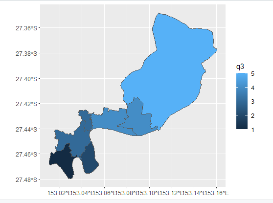
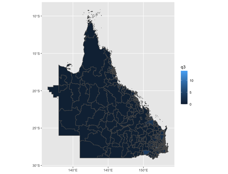
One small additional question, if I may, how would I go about inverting the colours used in the legend? Or, alternatively (if it is easier) having the rest of the map of Queensland displayed?
In the first instance, I mapped all Queensland postcodes using the method you suggested and the postcodes where 0 respondents came from appears very dark (see attached). I think inverting the legend colours (or having 0 appear as white or transparent) would make it a lot easier to see where respondents have come from - especially at the lower end of the scale.