Plotting values from a function

Try this block:

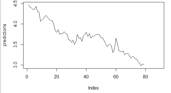
The interest rate data can be found on https://fred.stlouisfed.org/graph/?g=NUh

Then you need to press Download button on the webpage (it should be downloaded in csv format)
And then:
library(readr)
Series<-read_csv("~/Downloads/MORTGAGE30US (3).csv"

# transform data to stationarity
  diffed = diff(Series, differences = 1)
  
  
  # create a lagged dataset, i.e to be supervised learning
  
  lags <- function(x, k){
    
    lagged =  c(rep(NA, k), x[1:(length(x)-k)])
    DF = as.data.frame(cbind(lagged, x))
    colnames(DF) <- c( paste0('x-', k), 'x')
    DF[is.na(DF)] <- 0
    return(DF)
  }
  supervised = lags(diffed, k)
  
  
  ## split into train and test sets
  
  N = nrow(supervised)
  n = round(N *0.66, digits = 0)
  train = supervised[1:n, ]
  test  = supervised[(n+1):N,  ]
  
  
  ## scale data
  normalize <- function(train, test, feature_range = c(0, 1)) {
    x = train
    fr_min = feature_range[1]
    fr_max = feature_range[2]
    std_train = ((x - min(x) ) / (max(x) - min(x)  ))
    std_test  = ((test - min(x) ) / (max(x) - min(x)  ))
    
    scaled_train = std_train *(fr_max -fr_min) + fr_min
    scaled_test = std_test *(fr_max -fr_min) + fr_min
    
    return( list(scaled_train = as.vector(scaled_train), scaled_test = as.vector(scaled_test) ,scaler= c(min =min(x), max = max(x))) )
    
  }
  
  
  ## inverse-transform
  inverter = function(scaled, scaler, feature_range = c(0, 1)){
    min = scaler[1]
    max = scaler[2]
    n = length(scaled)
    mins = feature_range[1]
    maxs = feature_range[2]
    inverted_dfs = numeric(n)
    
    for( i in 1:n){
      X = (scaled[i]- mins)/(maxs - mins)
      rawValues = X *(max - min) + min
      inverted_dfs[i] <- rawValues
    }
    return(inverted_dfs)
  }
  
  
  Scaled = normalize(train, test, c(-1, 1))
  
  y_train = Scaled$scaled_train[, 2]
  x_train = Scaled$scaled_train[, 1]
  
  y_test = Scaled$scaled_test[, 2]
  x_test = Scaled$scaled_test[, 1]
  
  ## fit the model
  
  dim(x_train) <- c(length(x_train), 1, 1)
  dim(x_train)
  X_shape2 = dim(x_train)[2]
  X_shape3 = dim(x_train)[3]
  batch_size = 1
  units = 1
  
  model <- keras_model_sequential() 
  model%>%
    layer_lstm(units, batch_input_shape = c(batch_size, X_shape2, X_shape3), stateful= TRUE)%>%
    layer_dense(units = 1)


  model %>% compile(
    loss = 'mean_squared_error',
    optimizer = optimizer_adam( lr= 0.02 , decay = 1e-6 ),  
    metrics = c('accuracy')
  )


  summary(model)
  
  nb_epoch = Epochs   
  for(i in 1:nb_epoch ){
    model %>% fit(x_train, y_train, epochs=1, batch_size=batch_size, verbose=1, shuffle=FALSE)
    model %>% reset_states()
  }
  
  
  L = length(x_test)
  dim(x_test) = c(length(x_test), 1, 1)
  
  scaler = Scaled$scaler

  predictions = numeric(L)
  for(i in 1:L){
    X = x_test[i , , ]
    dim(X) = c(1,1,1)
    # forecast
    yhat = model %>% predict(X, batch_size=batch_size)
    
    # invert scaling
    yhat = inverter(yhat, scaler,  c(-1, 1))
    
    # invert differencing
    yhat  = yhat + Series[(n+i)] 
    
    # save prediction
    predictions[i] <- yhat
  }

Ok and what does predictions look like after you've done that?

(just enter predictions at the console or add it as a new line after your code above, and then Ctrl+Enter on that line to run)

It looks like the following:

> predictions
 [1] 4.474622 4.407538 4.389131 4.353723 4.358029 4.429131 4.312132 4.299131 4.063708
[10] 4.099131 4.133164 4.189131 4.205284 4.159131 4.110012 4.089131 4.079131 3.987404
[19] 3.839131 3.798492 3.859131 3.749131 3.769131 3.767892 3.814816 3.769131 3.758436
[28] 3.619131 3.602132 3.551570 3.599131 3.506316 3.558345 3.749131 3.653164 3.669131
[37] 3.573708 3.709131 3.739524 3.799131 3.695284 3.769131 3.658980 3.699131 3.699131
[46] 3.728980 3.749131 3.740556 3.739131 3.659131 3.667892 3.600088 3.529131 3.448980
[55] 3.489131 3.503164 3.469131 3.303164 3.379131 3.660012 3.508709 3.349131 3.335284
[64] 3.321360 3.340655 3.249131 3.276316 3.289377 3.236669 3.169131 3.199131 3.199543
[73] 3.142826 3.148801 3.080307 3.049131 2.977404 3.029131 3.006316       NA       NA
[82]       NA       NA       NA       NA       NA       NA       NA       NA

Visualizing that:

image

But I still don't understand how to get this plot:
image

1 Like

My advice is: keep trying things, keep reading, keep learning.
You won't learn much by expecting others to do all your work for you.

Could you clarify whether you're trying to replicate the formatting of that plot, or are you concerned because your data doesn't look like it's the same as the author's data?

I don't know how to fix the latter issue since I'm really unfamiliar with time series forecasting. But if it's the former, then your question would be more about how to use R's various plot commands. From the format of this plot, it looks like it was plotted using the base R plot function, which I'm not personally familiar with enough to help you (though there is a helpful article here among other things). I can help more if you're interested in using the ggplot2 package to make a plot.

But I'm guessing from your questions that what you're concerned about is the data itself, and unfortunately that's out of my wheelhouse...

1 Like

I was interested in plotting this picture somehow:

image

But there was no such a code line in the listing above, which could be used to create this plot.That's why I asked for help.

this was a fine question, that you did not directly answer.
do you want to reproduce this picture down to the exact placement of every point in the chart, or is it the features of the chart in general that interest you . like having a legend, having 3 lines etc.

I'd like to to reproduce this picture down to the exact placement of every point in the chart.

ok, then please provide a version of the code which is as complete as you can make it, as francisbarton and I have pointed out, the original script you are following is incomplete, k is unset, epochs is unset.
You will probably need to take the time to read the tutorial text, to determine how to complete the script.
run it step by step so that you can be awake to errors and missing parts.

When you get to a specific problem which is reproducible then you can share it with us in the ways detailed to you, and the forum users can provide you help over a concrete issue.

2 Likes

This topic was automatically closed 21 days after the last reply. New replies are no longer allowed.

If you have a query related to it or one of the replies, start a new topic and refer back with a link.