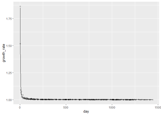
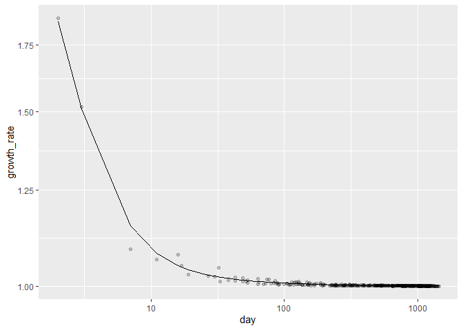
I am able to get a pretty good fit. Looks good even from log-log perspective.
The critical pieces!
- model log(growth - 1). To capture the exponential relationship, it's important to have a quantity that goes towards zero so when we take the log, the log continues to decrease through the orders of magnitude 10^-1, 10^-2, 10^-3, ...
- weight the regression with the growth rate so it places greater leverage on the first couple hundred days where growth is high. Because the fit is now minimizing sum of squares of the log, we don't want it to focus so much on the very small growth rates
- I have a poly(3) in the regression, but it's not that necessary. Looks ok with only poly(1)
library(tidyverse)

df <- structure(list(day = c(668, 228, 872, 715, 159, 337, 935, 278,
822, 808, 647, 272, 169, 929, 507, 38, 241, 776, 836, 477, 3,
503, 729, 654, 526, 341, 239, 447, 608, 732, 829, 225, 246, 553,
641, 699, 805, 434, 796, 136, 243, 197, 319, 287, 751, 570, 537,
440, 155, 888, 283, 72, 778, 795, 148, 765, 74, 309, 63, 286,
942, 89, 997, 864, 64, 808, 130, 895, 824, 2, 152, 545, 250,
529, 907, 909, 11, 941, 168, 358, 880, 315, 771, 647, 528, 295,
894, 269, 739, 467, 439, 325, 504, 111, 106, 604, 493, 549, 608,
913, 496, 588, 30, 695, 350, 277, 688, 427, 353, 83, 118, 379,
257, 915, 187, 548, 352, 828, 793, 647, 501, 649, 830, 105, 674,
400, 998, 33, 753, 85, 950, 16, 395, 418, 314, 711, 978, 852,
219, 701, 324, 718, 790, 619, 471, 328, 27, 88, 576, 849, 690,
338, 392, 389, 123, 806, 945, 847, 960, 329, 345, 657, 43, 123,
493, 502, 650, 534, 230, 460, 281, 920, 861, 776, 114, 908, 645,
497, 849, 503, 429, 91, 111, 313, 433, 882, 703, 611, 792, 160,
128, 277, 187, 486, 321, 528, 150, 571, 153, 382, 420, 193, 529,
118, 513, 711, 108, 550, 489, 709, 243, 473, 32, 984, 493, 661,
494, 570, 812, 887, 17, 77, 126, 546, 137, 525, 400, 238, 232,
494, 143, 151, 251, 285, 53, 150, 70, 984, 135, 805, 284, 19,
52, 366, 53, 747, 63, 393, 121, 79, 223, 767, 532, 244, 875,
981, 531, 92, 931, 49, 798, 304, 751, 49, 245, 763, 188, 591,
754, 365, 128, 86, 132, 786, 271, 938, 759, 198, 716, 601, 43,
7, 482, 299, 168, 779, 201, 308, 237, 99, 195, 1000, 397, 897,
261, 921, 732, 174, 563, 636, 1293, 1199, 1196, 1188, 1156, 1021,
1077, 1123, 1200, 1264, 1322, 1128, 1150, 1206, 1408, 1194, 1162,
1075, 1155, 1108, 1091, 1059, 1126, 1008, 1015, 1073, 1024, 1171,
1096, 1218, 1022, 1286, 1063, 1172, 1047, 1411, 1386, 1190, 1341,
1051, 1017, 1010, 1219, 1190, 1193, 1038, 1006, 1171, 1422, 1162,
1186, 1147, 1195, 1366, 1162, 1376, 1097, 1353, 1008, 1010, 1010,
1037, 1225, 1155, 1208, 1258, 1309, 1241, 1225, 1111, 1041, 1244,
1354, 1092, 1022, 1041, 1068, 1048, 1205, 1327, 1057, 1233, 1173,
1075, 1055, 1238, 1256, 1442, 1210, 1056, 1227, 1050, 1009, 1085,
1304, 1056, 1145, 1016, 1130, 1202), growth_rate = c(1, 1.00306502480229,
1, 1.00076851094002, 1.00148339803649, 1.00045123354242, 1.00020383148751,
1.00040965825011, 1, 1.00031779508266, 1.00066482023658, 1.00346513143248,
1.00425818538852, 1.0000656266777, 1.0001181890034, 1.01397743783103,
1.00139112715821, 1.00081959407673, 1.00009809095611, 1.00044236058947,
1.51727840805678, 1.00121675720201, 1.00008407903631, 1.0002592753402,
1.000030898582, 1.00018747698804, 1.00076380264933, 1.00036102684816,
1.00014528643822, 1.00062904941809, 1.00035187773298, 1.00111580249086,
1.00128571600603, 1.00016768160482, 1.00031901973645, 1.00023357797553,
1, 1.00041471510241, 1.00035864164816, 1.00240475926205, 1.00171028989878,
1.00424915891236, 1.00132476644926, 1.00221292841008, 1.00050907600983,
1.00044491397686, 1.00159525492273, 1.00180564684984, 1.00736657558218,
1, 1.0026255455024, 1.00522416568146, 1.00053636280677, 1.00036357279992,
1.00848394039131, 1.00006750976761, 1.01480026218821, 1.00284373740064,
1.00450411011131, 1.00221965194253, 1, 1.00539973548843, 1, 1.0005005471049,
1.0090122482097, 1, 1.00323230127301, 1.00032245565711, 1.00011354681804,
1.86253085002583, 1.00493992498232, 1.00241870746302, 1.00078006797611,
1.00098571121886, 1.00020587722401, 1, 1.06357635769067, 1.00002460995387,
1.00391720899917, 1.00119656881149, 1, 1.00107863162601, 1.00105245561527,
1.00008689169125, 1.0012783975488, 1.00154555116813, 1.00007359702218,
1.00084802657738, 1.00041660475254, 1.00011183062243, 1.00063625619285,
1.00135232882137, 1.00028938223461, 1.00315936176759, 1.00532364235978,
1.00030657799902, 1.00061342100673, 1.00030571104406, 1.00011715885948,
1, 1.00047974561815, 1.00025430105801, 1.02198934501457, 1.00010416687303,
1.00059014062243, 1.00047780779104, 1.00002874641645, 1.00111112119003,
1.00048837107964, 1.00754570558638, 1.00755154435772, 1.00254002012421,
1.00159784391408, 1.00007543627185, 1.00378184040293, 1.0003705762736,
1.00036115588121, 1.00022933557137, 1.00029709263616, 1.00009829460504,
1.00140576471426, 1, 1.00005859317971, 1.00525400638917, 1.00011859424543,
1.00056320336456, 1.00035496874922, 1.00990917838274, 1.00003017505772,
1.01216605816059, 1.00009508876079, 1.07550081281054, 1.0009053688873,
1.00033679896333, 1.00256186904405, 1.00024334207759, 1, 1.00006156466836,
1.0010976624319, 1.00012077834143, 1.00128712135851, 1.0001649556448,
1, 1.00026425686049, 1.00101428907282, 1.0018129199355, 1.0232877524855,
1.00781265091469, 1.00088597626466, 1.00009409356407, 1.00015668455482,
1.00207944494908, 1.0008364573296, 1.00025217525085, 1.00851816270978,
1.00016567699951, 1.0005450520462, 1, 1.00005352201724, 1.00265963863935,
1.00278084396241, 1.00039100408185, 1.0119269039859, 1.00348007368147,
1.00028324293254, 1.00093475581609, 1, 1.00049601640004, 1.00093369723894,
1.00060643539062, 1.00045179198477, 1.0001781622325, 1.00046194521224,
1, 1.00837269520819, 1.00020635263389, 1, 1.00059134502924, 1.00037811956032,
1.00041897791628, 1.00042567344896, 1.00315548828686, 1.00468000407093,
1.00117636662781, 1.00060407694, 1.00024651907264, 1.00040214420152,
1.00026572826846, 1, 1.00339182682076, 1.00677033400408, 1.00155795560629,
1.00709197798949, 1.00038408589383, 1.00044811349183, 1.00130624808202,
1.00213573137913, 1.00033829641388, 1.00181882251488, 1.00135268084575,
1.00021867236035, 1.00124421720953, 1.00167528270764, 1.00177999673699,
1.00111286906933, 1.00010382083562, 1.00281412834574, 1.00056084643116,
1.0003141068177, 1.00008783630833, 1.00295297113833, 1.00164418951503,
1.04254942398587, 1.00003463339853, 1.00026114582086, 1.00050325855951,
1.00027372250255, 1.00087794701574, 1, 1.00013019716725, 1.04849400865707,
1.01576530751161, 1.00464667740791, 1.00018645212712, 1.00232488088618,
1.00004828157946, 1.00003981436502, 1.00154051691592, 1.00300130371862,
1.00123014317303, 1.00178350354365, 1.00280125310909, 1.00058260459095,
1.00046312111938, 1.01338850447998, 1.00324092586586, 1.00435413084373,
1.00045526312721, 1.00239458582682, 1, 1.00072778216623, 1.02606789744901,
1.01114042578054, 1.00064178777718, 1.0070741027695, 1.00012247290823,
1.01674249234518, 1.00242915312699, 1.00914195421065, 1.00600241912814,
1.00186581948127, 1, 1.0009766510536, 1.00356182186649, 1.00061069533127,
1.0004239892255, 1, 1.00423354957881, 1, 1.01840023022722, 1.00014520016924,
1.00092286729759, 1.00006763577849, 1.01050940078589, 1.00083492872673,
1, 1.00212321384912, 1.00042771571448, 1.00005841382969, 1.00091286897932,
1.01020966954758, 1.00636232332844, 1.00629472490287, 1.00006023350623,
1.0006479378345, 1, 1, 1.00192163655976, 1.00037288252448, 1.00079827070308,
1.02036948481831, 1.08953748979677, 1.00005419459345, 1.00091099942311,
1.00158239355759, 1.00056725169743, 1.00254767904885, 1.00323409855214,
1.00082718448862, 1.00453370970986, 1.000723554716, 1.00017946087637,
1.00177142955793, 1.00002646875663, 1.00176656474078, 1.00062703527375,
1.00005493403402, 1.00516938013927, 1.00041653082443, 1.00014928977913,
1.00020721162875, 1, 1, 1, 1.00006564860028, 1, 1, 1, 1, 1.00003044890406,
1, 1, 1, 1, 1, 1, 1, 1.0001045870866, 1.0000969223039, 1.00003558158276,
1, 1.00014456034634, 1, 1.00006005834686, 1.00001996732182, 1,
1, 1, 1.00006796560531, 1.00002505991713, 1.00033215470201, 1.00025086529074,
1, 1, 1.00005211550219, 1, 1, 1, 1, 1.00005113850633, 1.00003684287429,
1.00007239452958, 1.00009072804825, 1, 1, 1, 1, 1.00018251149956,
1, 1, 1, 1, 1, 1, 1, 1, 1.00002144750158, 1, 1.00002257182718,
1, 1.0001890858105, 1, 1, 1, 1, 1, 1, 1.00001721483368, 1.00005676253354,
1.00012229728215, 1, 1.00020620900577, 1, 1, 1, 1, 1.00044288582059,
1.00002461203578, 1, 1.00008842939096, 1.00006595081859, 1, 1.00007436380507,
1, 1, 1, 1, 1, 1, 1, 1, 1, 1.00080787992677, 1, 1, 1.00013030856866,
1.00022073762073, 1, 1.00001973205065, 1.00005050803594)), row.names = c(NA,
-400L), class = "data.frame")

# log-log with growth - 1 is approx. linear
print(
  df %>% ggplot() + aes(day, growth_rate - 1) + geom_point() +
    scale_x_log10() + scale_y_log10()
)
#> Warning: Transformation introduced infinite values in continuous y-axis
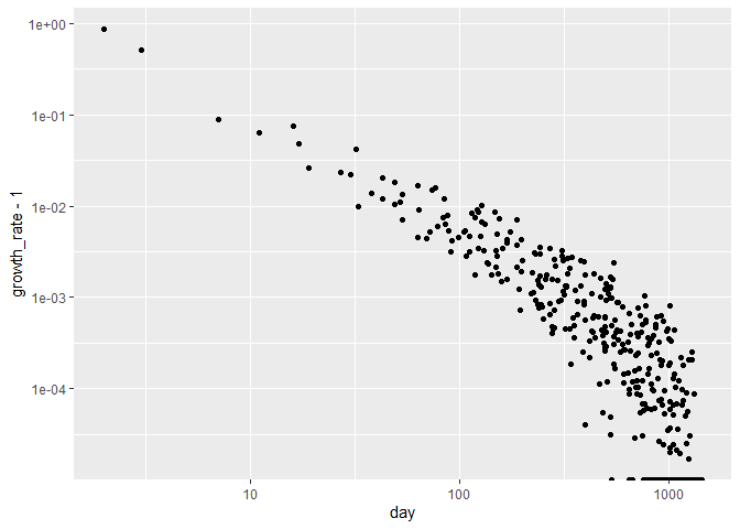
# the reason why we need to subtract 1 is so growth can continue to decrease through
# orders of magnitude 10^-1, 10^-2, etc.

# add columns for the transformed variables
df  <- df %>%
  mutate(growth_rate_m1 = growth_rate - 1, day_plus_3 = day + 3)

# filtered so we can model
dfm <- df %>% filter(growth_rate > 1)

# fit model and add predicted growth to df
model <- lm(
  log(growth_rate_m1) ~ poly(log(day_plus_3), 3),
  data = dfm,
  weights = growth_rate_m1 # scale high values more
)
summary(model) %>% print()
#>
#> Call:
#> lm(formula = log(growth_rate_m1) ~ poly(log(day_plus_3), 3),
#>     data = dfm, weights = growth_rate_m1)
#>
#> Weighted Residuals:
#>       Min        1Q    Median        3Q       Max
#> -0.156213 -0.019200 -0.010042  0.005349  0.143044
#>
#> Coefficients:
#>                            Estimate Std. Error t value Pr(>|t|)
#> (Intercept)                -6.76221    0.06968 -97.049  < 2e-16 ***
#> poly(log(day_plus_3), 3)1 -26.26473    0.96626 -27.182  < 2e-16 ***
#> poly(log(day_plus_3), 3)2  -2.83995    0.66531  -4.269 2.63e-05 ***
#> poly(log(day_plus_3), 3)3  -3.43207    0.32168 -10.669  < 2e-16 ***
#> ---
#> Signif. codes:  0 '***' 0.001 '**' 0.01 '*' 0.05 '.' 0.1 ' ' 1
#>
#> Residual standard error: 0.02707 on 305 degrees of freedom
#> Multiple R-squared:  0.9805, Adjusted R-squared:  0.9803
#> F-statistic:  5107 on 3 and 305 DF,  p-value: < 2.2e-16
df <- df %>% mutate(pred_growth = exp(predict(model, df)) + 1)

# plot
print(
  df %>%
  ggplot() +
  geom_point(aes(day, growth_rate), alpha = 0.2) +
  geom_line(aes(day, pred_growth))
)
print(
  df %>%
    ggplot() +
    geom_point(aes(day, growth_rate), alpha = 0.2) +
    geom_line(aes(day, pred_growth)) +
    scale_x_log10() + scale_y_log10()
)
Created on 2022-02-03 by the reprex package (v2.0.1)