Hey guys! I need a help on a interpretation of a out of a code statistics' linear method. What does the results mean such as "F(1,3) = 4.195, p = 0.133 R² = 0.583 Adj. R² = 0.444" and, specially, the last table on the out of the code?
OUT:
´´´ >
Carregando pacotes
#explorar dados
library(tidyverse)
library(learnr)
library(openintro)
library(gapminder)
library(gt)
library(patchwork)
library(broom)
library(dplyr)
library(WriteXLS)Carregando o dataset
library(readxl)
pmm <- read_excel("pmm.xlsx")
View(pmm)library(readxl)
pmmestrangeiros <- read_excel("pmmestrangeiros.xlsx")
View(pmmestrangeiros)library(readxl)
combpmmatt <- read_excel("combpmmatt.xlsx")
View(combpmmatt)Observando o dataset
glimpse(pmm)
Rows: 58,042
Columns: 5
NU_INSCRICAO <dbl> 421026, 459595, 459558, 497387, 497446, 495746, 4… NO_PESSOA "FABIO MARLON MARTINS FRANCA", "JESSE DE PAULA", …
CO_MUNICIPIO_IBGE_ATUACAO <chr> "520530", "432300", "330170", "530010", "230440",… SG_UF_ATUACAO "GO", "RS", "RJ", "DF", "CE", "SE", "PR", "MA", "…
$ DS_LOCAL_ATUACAO "CAVALCANTE", "VIAMAO", "DUQUE DE CAXIAS", "BRASI…Observando o dataset
glimpse(pmmestrangeiros)
Rows: 269
Columns: 2
NO_PESSOA <chr> "ADISMARY CEBALLOS INFANTE", "ADRIANA YASMINE BOLIVAR TRIGO V… NACIONALIDADE "CUBA", "BOLIVIA", "VENEZUELA", "URUGUAI", "ARGENTINA", "ARGE…###comparando
combpmm <- left_join(pmm,pmmestrangeiros, by = c("NO_PESSOA"))###mudando nacionalidade vazia porque os estrangeiros ja tem preenchimento
combpmm$NACIONALIDADE[which(is.na(combpmm$NACIONALIDADE))] <- "BRASIL"
#Criando gráfico
ggplot(data = combpmm, aes(x = SG_UF_ATUACAO)) +
- geom_bar()
combpmmatt %>%
- group_by(REGIAO) %>%
- summarise(quantidade = n())
A tibble: 5 × 2
REGIAO quantidade
1 CENTRO-OESTE 4103
2 NORDESTE 22795
3 NORTE 6779
4 SUDESTE 15951
5 SUL 8414
library(readxl)
promod_ <- read_excel("promod.xlsx")
View(promod_)promod__summary <- promod_ %>%
- summarise(
-
mean = round(mean(MedicosPMM), 1), -
med = round(median(MedicosPMM), 1), -
mode = 80, -
var = round(var(MedicosPMM), 2), -
sd = round(sd(MedicosPMM), 2), -
iqr = round(IQR(MedicosPMM), 2) - )
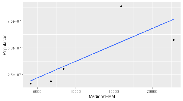
promod_ %>%
- ggplot(aes(x = MedicosPMM, y = Populacao)) +
- geom_point() +
- geom_smooth(method = "lm", se = FALSE)
geom_smooth()using formula 'y ~ x'
modmedicos <- lm(Populacao~MedicosPMM, data = promod_)
summary(modmedicos) #Parâmetros do modelo
Call:
lm(formula = Populacao ~ MedicosPMM, data = promod_)
Residuals:
1 2 3 4 5
-2807420 -19316534 -8853681 33330571 -2352936
Coefficients:
Estimate Std. Error t value Pr(>|t|)
(Intercept) 6716696 20192650 0.333 0.761
MedicosPMM 3070 1499 2.048 0.133
Residual standard error: 22920000 on 3 degrees of freedom
Multiple R-squared: 0.5831, Adjusted R-squared: 0.4441
F-statistic: 4.195 on 1 and 3 DF, p-value: 0.133
confint(modmedicos, level = 0.95) #intervalos de confiança do modelo
2.5 % 97.5 %
(Intercept) -57545327.970 70978719.264
MedicosPMM -1699.918 7839.342summ(modmedicos, confint = T, digits = 3, ci.width = .95) #Parâmetros do modelo (expostos de outra forma)
MODEL INFO:
Observations: 5
Dependent Variable: Populacao
Type: OLS linear regression
MODEL FIT:
F(1,3) = 4.195, p = 0.133
R² = 0.583
Adj. R² = 0.444
Standard errors: OLS
Est. 2.5% 97.5% t val. p
(Intercept) 6716695.647 -57545327.970 70978719.264 0.333 0.761
MedicosPMM 3069.712 -1699.918 7839.342 2.048 0.133
export_summs(modmedicos, scale = F, digits = 5)
─────────────────────────────────────────────────
Model 1
─────────────────────────
(Intercept) 6716695.64677
(20192649.75832)
MedicosPMM 3069.71183
(1498.73065)
─────────────────────────
N 5
R2 0.58305
─────────────────────────────────────────────────
*** p < 0.001; ** p < 0.01; * p < 0.05.
Column names: names, Model 1 ´´´
FINAL GRAPHIC: