Please, I need help with generating temperature maps in R. I have a grided temperature data for a region in West Africa and want to draw a temperature map for the region alone without showing the outlying areas. Any thought on how to do this
This will depend on format of your data. Gridded measurements like temperature you describe, or remote sensing (satellite) data are often approached via the package raster.
Rasters are easily clipped via raster::mask().
Or you can use general vector maps - sf is currently the best practice, but you will encounter the older package sp a lot in older online materials; it may be obsolete now, but it lived a long and happy life.
Intersection of a grid and a sf object representing boundaries is done via sf::st_intersection().
You would of course need to link the grid to your data and use your favorite plotting library (I suggest ggplot2, but I am not a prude) to draw the map.
Thanks for the prompt response and suggestion for the reprex. Tried it and I hope what I did was the right the thing (concerning the reprex).
So I have temperature data for West Africa and managed to extract the portion for Ghana using grid-specific location for Ghana thus producing the longitudes, latitudes and temperature recorded in that region from 1980 to 2010. Now, I want to create map for this region with the shape of Ghana displayed. Tried merging Ghana shapefiles and the data frame I generated from the grid location to create the map but I received error messages. Unfortunately, I did not record that error message in this reprex. But below is what I've done so far. Please let me know if my reprex worked. Also, I tried the sf package but it does not install in my RStudio
library(dplyr)
#>
#> Attaching package: 'dplyr'
#> The following objects are masked from 'package:stats':
#>
#>     filter, lag
#> The following objects are masked from 'package:base':
#>
#>     intersect, setdiff, setequal, union
the temperature data was extracted from a netcdf file for the location I needed, which in this case is Ghana. the whole region was for west africa but am only analysing the region of Ghana. tried the sf package but could not install the package in my RStudio. I even tried merging Ghana's shapefile with the grid data extracted for Ghana to generate my map but returned an error message. tried this reprex, kindly check if it contains all my code and do share your thoughts on it.
There is a problem with your reprex, apparently you just made it with the first line of your code (that is all we can see), could you pleas check on this? maybe this reprex guide would be easier to understand for you.
the link is very helpful but I think posting my code (what I've done so far will provide a good overview of my problem). Is it possible I could just copy and paste my code directly and probably share a link to the data am working with?
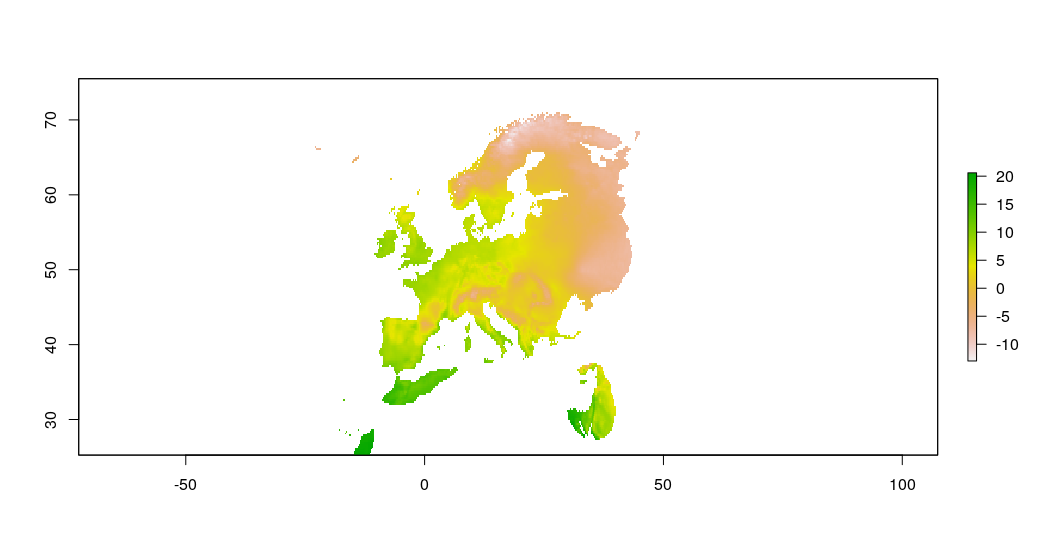
I can not reproduce your code, but allow me to illustrate the approach on a similar use case; I have used temperature data from Copernicus and cropped it to shape of the Czech Republic from GADM.
This approach requires only two packages (raster and sf) + tidyverse, just because :))
It uses two steps:
remove the extra data points via raster::mask()
crop the file down to size via raster::crop()
library(tidyverse) # because tidyverse :)
library(raster) # raster spatial data processing
library(sf) # vector spatial data processing
data <- raster("./src/tg_0.25deg_day_2019_grid_ensmean.nc") # your ncdf file
borders <- readRDS("./src/gadm36_CZE_0_sf.rds") # country borders in sf format
plot(data) # the big picture
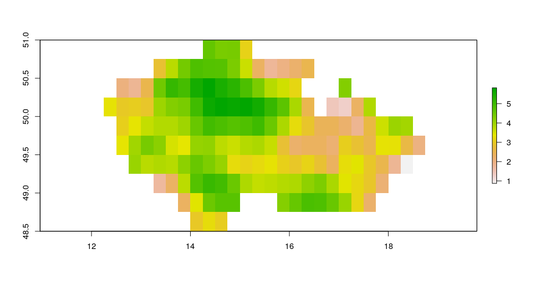
data_masked <- mask(data,borders) %>% # mask the unwanted areas
crop(borders) # crop to shape
plot(data_masked) # the small picture
Many thanks for your help. The information was very useful. Unfortunately, the "sf" library fails to load in my RStudio though the programme has been installed. Thus, I used the "sp" function which did work. Below is my code
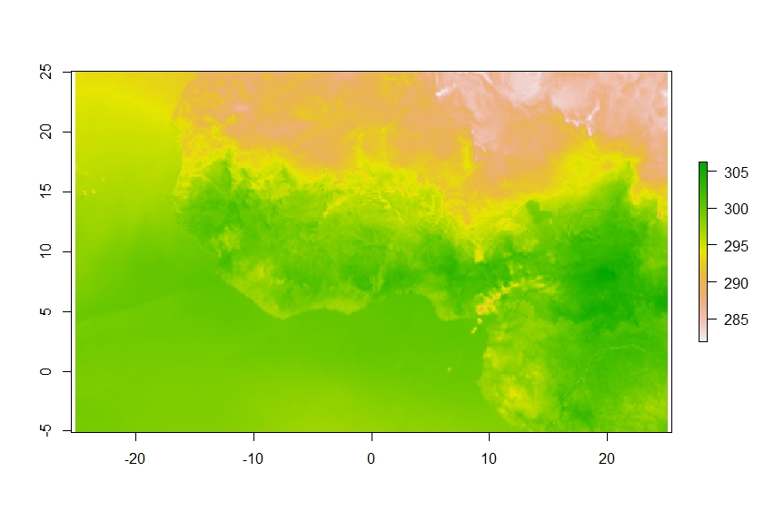
data <- raster("wa12clmN_eraint_ctrl_tas_1980_2009_DAYMEAN.nc") # your ncdf file
borders <- readRDS("F:/DISSERTATION FOLDER/rcm_data/gadm36_GHA_1_sp.rds") # country borders in sf format
plot(borders)
plot(data) # the big picture
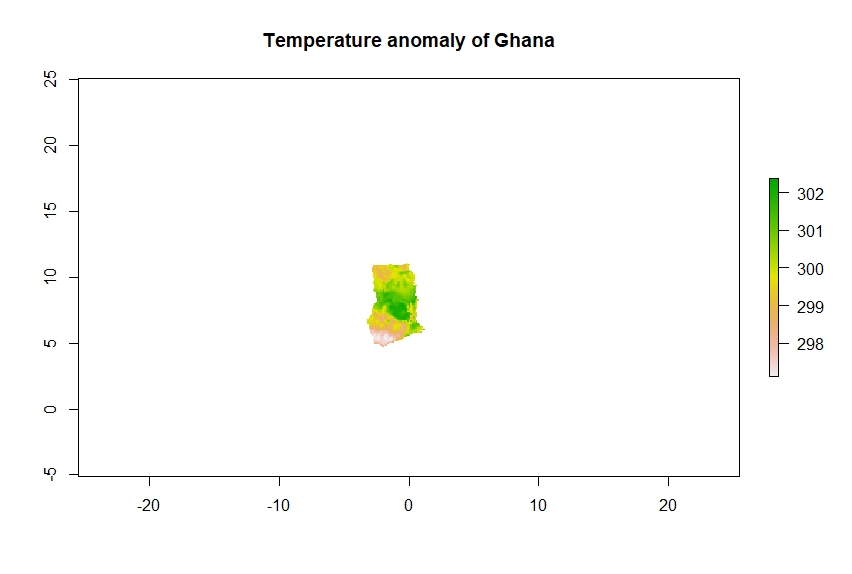
data_masked <- mask(data, borders) ##mask the unwanted areas
tempgh <- plot(data_masked, main = "Temperature anomaly of Ghana") # the small picture
With these outputs, I can rework my data and hopefully produce better temperature maps. Really grateful for your help and would reach out should I have any dilemma
The {sp} is a good package, and it did the job. You may want to persevere with the newer {sf} package though, as it is the current best practice and allows the use of goodies like geom_sf, which I am sure would make your dissertation more appealing.
The reason the map retains the original extent is that you did not crop it after masking.
Consider adding the command like this:
data <- raster("wa12clmN_eraint_ctrl_tas_1980_2009_DAYMEAN.nc") # your ncdf file

borders <- readRDS("F:/DISSERTATION FOLDER/rcm_data/gadm36_GHA_1_sp.rds") # country borders in sp format

plot(borders)

plot(data) # the big picture

data_masked <- mask(data, borders) # mask the unwanted areas
data_masked <- crop(data_masked, borders) # crop the image down to size

tempgh <- plot(data_masked, main = "Temperature anomaly of Ghana") # the small picture