Hello,
I have a data set over five years of 24 different products.
I would like to create a time series forecasting plot to look at the purchase history of these 24 products.
Can I produce an out-put plot for each product?
Thanks!
Hello,
I have a data set over five years of 24 different products.
I would like to create a time series forecasting plot to look at the purchase history of these 24 products.
Can I produce an out-put plot for each product?
Thanks!
Yep – I'm not sure what exactly you mean by out-plot plot, but you can certainly plot all of them together using facet_wrap() (or grid),
https://www.r-graph-gallery.com/280-use-faceting-for-time-series-with-ggplot2/
or make many plots by writing a function and passing in the product variable with quasiquotation:
Many other ways too, I imagine. But, to answer your question: yes.
Mara:
That is exactly what I need.
I will post more follow-up questions on this topic later.
You guys have been helpful.
Thanks, team!
There is a new package called TSstudio. It can do some really cool plots for time series and might serve your purpose well. Check the package intro
https://cran.r-project.org/web/packages/TSstudio/vignettes/TSstudio_Intro.html
(I fee the questions itself and the used tags are not matching well with the intended question)
rahmed:
Thank you, sir!
I corrected my post's title.
if you're doing time series forecasting then you should likely look at the forecast package from RJ Hyndman.
His book, Forecasting Principles and Practice is freely available online: Forecasting: Principles and Practice (2nd ed)
Here's an example of building an example time series model and associated plots:
library(forecast)
library(fpp2)
#> Loading required package: ggplot2
#> Loading required package: fma
#> Loading required package: expsmooth

a10 %>%
  BoxCox.lambda() ->
  lambda

a10 %>%
  BoxCox(lambda) %>%
  auto.arima() ->
  fit

print(fit)
#> Series: .
#> ARIMA(3,0,3)(0,1,1)[12] with drift
#>
#> Coefficients:
#>           ar1      ar2     ar3     ma1     ma2      ma3     sma1   drift
#>       -0.0607  -0.0007  0.7459  0.0751  0.2973  -0.4682  -0.8276  0.0126
#> s.e.   0.1207   0.1087  0.0966  0.1440  0.1246   0.1357   0.0663  0.0003
#>
#> sigma^2 estimated as 0.006168:  log likelihood=213.52
#> AIC=-409.03   AICc=-408.04   BIC=-379.72
checkresiduals(fit, plot=TRUE)

#>
#>  Ljung-Box test
#>
#> data:  Residuals from ARIMA(3,0,3)(0,1,1)[12] with drift
#> Q* = 20.172, df = 16, p-value = 0.2126
#>
#> Model df: 8.   Total lags used: 24
fit %>% forecast() %>% autoplot()
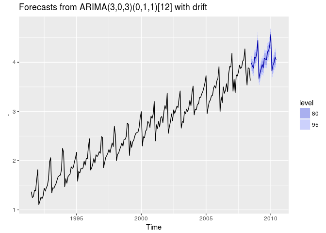
Created on 2018-06-26 by the reprex package (v0.2.0).
I am not sure about the question from the beginning as it is apparently a plotting problem with mix of forecasting requirement. Also the accepted solution for the question is based on plotting type solution.
As @jdlong suggested forecast package can be used for uni-variate forecasting and plotting. If 24 products are related and co-variance are important to consider in forecasting possibly one need to go beyond. Yet again the solution come from the research group led by Prof. Rob Hyndman. His hts package can be used for such purpose. Package intro can be found in this link.
awesome package, interactive too. but I didn't see any candlecharts there and any rolling funtions like Dygraph does.
But it's awesome. and could be huge going forward.
great point about hts, @rahmed. Here's a few possibly helpful links:
Chapter 10 "Forecasting hierarchical or grouped time series" from Forecasting Principles and Practice
Hyndman's lecture slides on the same topic: https://robjhyndman.com/nyc2018/3-3-Hierarchical.pdf