Timeserie (date_time) scatterplot

jrkrideau · February 28, 2023, 5:01pm

Looks promising. We will have to see what Pomwene thinks.

I've been experimenting with a day-by-day approach but at the moment it is in the "Brute Strength & Stupidity* level of coding.

library(tidyverse); 
library(data.table)
library(lubridate); 
library(rio);
library(patchwork)


dat1  <- import("Pomwene_R.xlsx"

D1125 <- dat1  |> filter(Date ==ymd("2022-11-25"))
D1126 <- dat1  |> filter(Date ==ymd("2022-11-26"))
D1127 <- dat1  |> filter(Date ==ymd("2022-11-27"))
D1128 <- dat1  |> filter(Date ==ymd("2022-11-28"))

 p1 <- D1125 %>%  ggplot(aes(DateTime, Conductance)) + geom_point() +
  geom_point( aes(colour= Leaf)) +
  ylim(0, 600) +
  geom_smooth(method = lm, se = F) +
  labs(x= "Datetime",  y= "Conductance") +
   ggtitle("Nov. 25")
 
 p2 <- D1126 %>%  ggplot(aes(DateTime, Conductance)) + geom_point(position = "jitter") +
   geom_point( aes(colour= Leaf)) +
   ylim(0, 600) +
   geom_smooth(method = lm, se = F) +
   labs(x= "Datetime",  y= "Conductance") +
   theme(legend.position="none")  +
   ggtitle("Nov. 26")
 
 p3 <- D1127 %>%  ggplot(aes(DateTime, Conductance)) + 
   ylim(0, 600) +
   geom_smooth(method = lm, se = F) +
   labs(x= "Datetime",  y= "Conductance") +
   theme(legend.position="none")  +
   ggtitle("Nov. 27")
 
 p4 <- D1128 %>%  ggplot(aes(DateTime, Conductance)) + geom_point() +
   geom_point( aes(colour= Leaf)) +
   ylim(0, 600) +
   geom_smooth(method = lm, se = F) +
   labs(x= "Datetime",  y= "Conductance") +
   theme(legend.position="none")  +
   ggtitle("Nov. 28")
 
 
  p1 + p2 + p3 + p4  + plot_layout(ncol = 2)

four_panal_plot.pdf (50.5 KB)

Pomwene · February 28, 2023, 5:56pm

This looks great, can we perhaps have one graph per day/per plant to see the variations, with time series on x-axis, which means the date and time all showing in 90 degree angle

jrkrideau · February 28, 2023, 6:14pm

If I understand you correctly, I do not see any reason why we could not have this. I am at the s in the "Brute Strength & Stupidity* level of coding at the moment, so it is just a matter of doing some automating to reduce the amount of code.

Pomwene · February 28, 2023, 6:16pm

I see what you have done here, ist possible to have this 6-time series on x-axis, eg 3 am, 7 am, 3 pm, 7 pm and 23p just as an example, also if we can rotate the x-axis to be vertical so that we can accommodate 6 time series,
also if we can give another shot to create this per plant per day, that will be great

Pomwene · February 28, 2023, 6:19pm

This looks great, can we perhaps have one graph per day/per plant to see the variations, with time series on x-axis, which means the date and time all showing in 90 degree angle

andresrcs · February 28, 2023, 9:02pm

That would be 32 panels, that level of overplotting will render the figure useless in my opinion. How about something like this?

library(tidyverse)
library(readxl)
library(hms)

url <- "https://www.dropbox.com/scl/fi/ya3twt4l1vvq9uwaphgvq/Pomwene_R.xlsx?dl=1&rlkey=ipw2rj8nucb904x28kymae3sn"
download.file(url, "sample_data.xlsx")

sample_df <- read_excel("sample_data.xlsx")

sample_df %>% 
    mutate(stage = case_when(
        Date <= '2022-11-27' ~ 'before',
        Date > '2022-11-27' & Date <= '2022-11-30' ~ 'after',
        .default = 'post'),
        stage = factor(stage, levels = c("before", "after", "post")),
        time = as_hms(DateTime)
    ) %>%
    ggplot(aes(x = time, y = Conductance, color = Plant_ID)) +
    geom_point() +
    geom_smooth(aes(group = stage), color = "blue", se = FALSE) +
    labs(x = "Time",  y = "Conductance") +
    scale_x_time(breaks = scales::breaks_width("1 hour"),
                 limits = c(0, 86.4E3),
                 expand = c(0, 0)) +
    facet_wrap(vars(stage), ncol = 1) +
    theme(legend.position = "bottom",
          axis.text.x = element_text(angle = 45, hjust = 1, vjust = 1))

^{Created on 2023-02-28 with reprex v2.0.2}

I also want to point out that you could try any plot variants you want on your own. I strongly recommend you read this book to learn how to wrangle and plot data yourself.

Pomwene · February 28, 2023, 9:21pm

Thank you for all your assistance, in the mean time i will go through this book. do you perhaps have a soft copy that you can share via email: paulinapwaw@gmail.com

jrkrideau · February 28, 2023, 10:47pm

I am still on the "Brute Strength and Stupidity" approach but I think this works although it has too much manual imput.

I am looking at the scale issue but I doubt that know enough about ggplot2 scales to be much help.

The first block of code creates 8 plots of DateTime X Conductance, one for each day. This means that you can do various comparisons as well as plot the entire series.

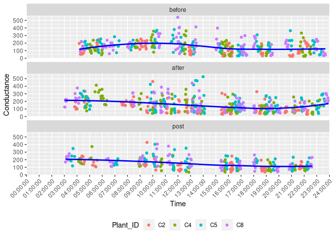
The second block is an example of doing the same for individual plants. It should be easy to extend to the same scale as the first block or you can just plot odd cobparisons that seem useful.

I hope this is of some use.

First Code Block

library(tidyverse); 
library(lubridate); 
library(rio); 
library(patchwork);

dat1  <- import("Pomwene_R.xlsx")

dng <- unique(dat1$Date)
dng <- ymd(substring(dng,1, 10))  ## Not really needed but it reduces typing

N25 <- dat1  |> filter(Date == dng[1])
N26 <- dat1  |> filter(Date == dng[2])
N27 <- dat1  |> filter(Date == dng[3])
N28 <- dat1  |> filter(Date == dng[4])
N29 <- dat1  |> filter(Date == dng[5])
N30 <- dat1  |> filter(Date == dng[6])
D06 <- dat1  |> filter(Date == dng[7])
D07 <- dat1  |> filter(Date == dng[8])

pN25  <- N25  %>%  ggplot(aes(DateTime, Conductance)) + geom_point() +
  geom_point(alpha=0.4, aes(colour = Leaf)) +
  ylim(0, 500) +
  geom_smooth(method = lm, se = F) +
  labs(x= "Date_time",  y= "Conductance") + ggtitle("Nov. 25")

pN26 <-  N26  %>%  ggplot(aes(DateTime, Conductance)) + geom_point()+
  geom_point(alpha=0.4, aes(colour= )) +  ylim(0, 500) + 
  geom_smooth(method = lm, se = F) +
  labs(x= "Date_time",  y= "Conductance") + ggtitle("Nov. 26") +
  theme(legend.position="none") 
  
pN27  <- N27  %>%  ggplot(aes(DateTime, Conductance)) + geom_point() +
    geom_point(alpha=0.4, aes(colour = Leaf)) +
    ylim(0, 500) +  geom_smooth(method = lm, se = F) +
    labs(x= "Date_time",  y= "Conductance") + ggtitle("Nov. 27")

pN28  <- N28  %>%  ggplot(aes(DateTime, Conductance)) + geom_point() +
  geom_point(alpha=0.4, aes(colour = Leaf)) +
  ylim(0, 500) + geom_smooth(method = lm, se = F) +
  labs(x= "Date_time",  y= "Conductance") + ggtitle("Nov. 28") +
  theme(legend.position="none") 

pN29  <- N29  %>%  ggplot(aes(DateTime, Conductance)) + geom_point() +
  geom_point(alpha=0.4, aes(colour = Leaf)) +
  ylim(0, 500) +   geom_smooth(method = lm, se = F) +
  labs(x= "Date_time",  y= "Conductance") + ggtitle("Nov. 29")

pN30  <- N30  %>%  ggplot(aes(DateTime, Conductance)) + geom_point() +
  geom_point(alpha=0.4, aes(colour = Leaf)) +
  ylim(0, 500) + geom_smooth(method = lm, se = F) +
  labs(x= "Date_time",  y= "Conductance") + ggtitle("Nov. 28") +
  theme(legend.position="none") 


pD06  <- D06  %>%  ggplot(aes(DateTime, Conductance)) + geom_point() +
  geom_point(alpha=0.4, aes(colour = Leaf)) +
  ylim(0, 500) + geom_smooth(method = lm, se = F) +
  labs(x= "Date_time",  y= "Conductance") + ggtitle("Dec. 06") +
  theme(legend.position="none") 

pD07  <- D07  %>%  ggplot(aes(DateTime, Conductance)) + geom_point() +
  geom_point(alpha=0.4, aes(colour = Leaf)) +
  ylim(0, 500) + geom_smooth(method = lm, se = F) +
  labs(x= "Date_time",  y= "Conductance") + ggtitle("Nov. 28") +
  theme(legend.position="none") 



pN25 + pN26 + pN27 + pN28 + plot_layout(ncol = 2)

# Compare First Day and Last Day Of the Study

pD06 + pD07

Second Code Block

library(tidyverse);  
library(lubridate); 
library(rio);
library(patchwork)

dat1  <- import("Pomwene_R.xlsx")

dng <- unique(dat1$Date)
dng <- ymd(substring(dng,1, 10)) 
pid <- c("C2", "C4", "C5", "C8")  # Plant_ID vector

test1 <- dat1  |> filter(Date == dng[1] & Plant_ID == pid[1])

ppf1  <- test1  %>%  ggplot(aes(DateTime, Conductance)) + geom_point() +
  geom_point(alpha=0.4, aes(colour = Leaf)) +
  ylim(0, 500) +
  geom_smooth(method = lm, se = F) +
  labs(x= "Date_time",  y= "Conductance") + ggtitle("Nov. 25, Plant", pid[1])

ppf1

Pomwene · February 28, 2023, 11:23pm

Very much helpful. I will consider definitely, for a beginner, this is very much easy to understand

jrkrideau · March 1, 2023, 3:53pm

I just noticed a new package {lemon} that may make life easier.

I had stuck theme(legend.position="none") in to get rid of extra legends but this looks like a better solution.

library(tidyverse); 
library(lubridate); 
library(rio); 
library(patchwork);
library(lemon); 

dat1  <- import("Pomwene_R.xlsx")

dng <- unique(dat1$Date)
dng <- ymd(substring(dng,1, 10))  ## Not really needed but it reduces typing

N25 <- dat1  |> filter(Date == dng[1])
N26 <- dat1  |> filter(Date == dng[2])
N27 <- dat1  |> filter(Date == dng[3])
N28 <- dat1  |> filter(Date == dng[4])
N29 <- dat1  |> filter(Date == dng[5])
N30 <- dat1  |> filter(Date == dng[6])
D06 <- dat1  |> filter(Date == dng[7])
D07 <- dat1  |> filter(Date == dng[8])

pN25  <- N25  %>%  ggplot(aes(DateTime, Conductance)) + geom_point() +
  geom_point(alpha=0.4, aes(colour = Leaf)) +
  ylim(0, 500) +
  geom_smooth(method = lm, se = F) +
  labs(x= "Date_time",  y= "Conductance") + ggtitle("Nov. 25")

pN26 <-  N26  %>%  ggplot(aes(DateTime, Conductance)) + geom_point()+
  geom_point(alpha=0.4, aes(colour= )) +  ylim(0, 500) + 
  geom_smooth(method = lm, se = F) +
  labs(x= "Date_time",  y= "Conductance") + ggtitle("Nov. 26") 
  
pN27  <- N27  %>%  ggplot(aes(DateTime, Conductance)) + geom_point() +
    geom_point(alpha=0.4, aes(colour = Leaf)) +
    ylim(0, 500) +  geom_smooth(method = lm, se = F) +
    labs(x= "Date_time",  y= "Conductance") + ggtitle("Nov. 27")

pN28  <- N28  %>%  ggplot(aes(DateTime, Conductance)) + geom_point() +
  geom_point(alpha=0.4, aes(colour = Leaf)) +
  ylim(0, 500) + geom_smooth(method = lm, se = F) +
  labs(x= "Date_time",  y= "Conductance") + ggtitle("Nov. 28")

pN29  <- N29  %>%  ggplot(aes(DateTime, Conductance)) + geom_point() +
  geom_point(alpha=0.4, aes(colour = Leaf)) +
  ylim(0, 500) +   geom_smooth(method = lm, se = F) +
  labs(x= "Date_time",  y= "Conductance") + ggtitle("Nov. 29")

pN30  <- N30  %>%  ggplot(aes(DateTime, Conductance)) + geom_point() +
  geom_point(alpha=0.4, aes(colour = Leaf)) +
  ylim(0, 500) + geom_smooth(method = lm, se = F) +
  labs(x= "Date_time",  y= "Conductance") + ggtitle("Nov. 28") 

pD06  <- D06  %>%  ggplot(aes(DateTime, Conductance)) + geom_point() +
  geom_point(alpha=0.4, aes(colour = Leaf)) +
  ylim(0, 500) + geom_smooth(method = lm, se = F) +
  labs(x= "Date_time",  y= "Conductance") + ggtitle("Dec. 06") 

pD07  <- D07  %>%  ggplot(aes(DateTime, Conductance)) + geom_point() +
  geom_point(alpha=0.4, aes(colour = Leaf)) +
  ylim(0, 500) + geom_smooth(method = lm, se = F) +
  labs(x= "Date_time",  y= "Conductance") + ggtitle("Dec. 07") 



## plot using {lemon}
grid_arrange_shared_legend(pN25, pN26, pD06, pD07, ncol = 2, nrow = 2)

andresrcs · March 3, 2023, 4:28am

2 posts were split to a new topic: Error loading tidyverse: ‘rlang’ 1.0.3 is already loaded, but >= 1.0.6 is required

system · March 24, 2023, 4:29am

This topic was automatically closed 21 days after the last reply. New replies are no longer allowed.

If you have a query related to it or one of the replies, start a new topic and refer back with a link.