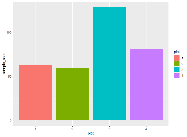
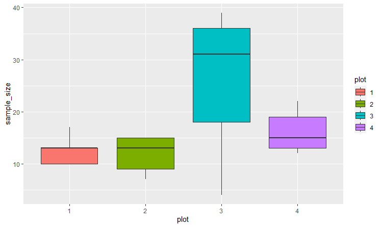
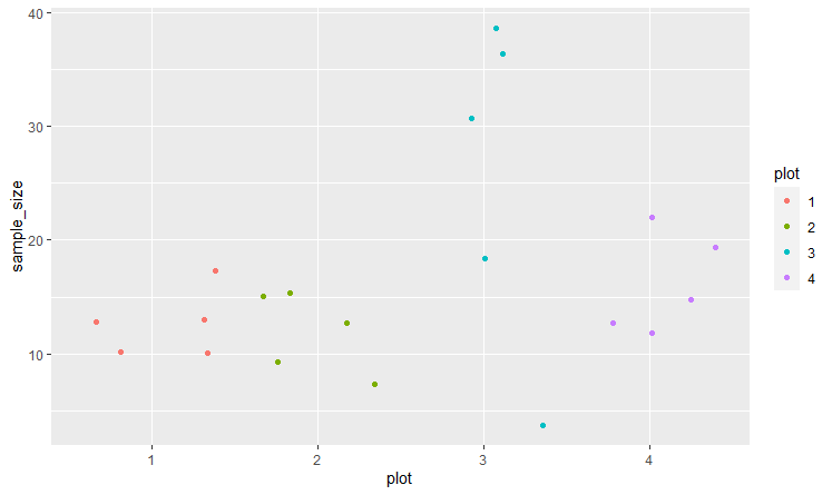
@jrkrideau that makes sense/ I see what your saying The data I have has 300 rows so hopefully this is OK to include here. (data below) I used dput() but dont know another way to make sharing this dataset smaller. here is is below. for date i have it as m/d/y. Im just having a hard time ordering things in the correct way to not get errors...
seed_count <-
structure(
list(
date = c(
"6/11/16",
"6/11/16",
"6/11/16",
"6/11/16",
"6/11/16",
"6/11/16",
"6/11/16",
"6/11/16",
"6/11/16",
"6/11/16",
"6/11/16",
"6/11/16",
"6/11/16",
"6/11/16",
"6/11/16",
"6/11/16",
"6/11/16",
"6/11/16",
"6/11/16",
"6/11/16",
"6/11/16",
"6/11/16",
"6/11/16",
"6/11/16",
"6/11/16",
"6/11/16",
"6/11/16",
"6/11/16",
"6/11/16",
"6/11/16",
"6/11/16",
"6/11/16",
"6/11/16",
"6/11/16",
"6/11/16",
"6/11/16",
"6/11/16",
"6/11/16",
"6/11/16",
"6/11/16",
"6/11/16",
"6/11/16",
"6/11/16",
"6/11/16",
"6/11/16",
"6/11/16",
"6/11/16",
"6/11/16",
"6/11/16",
"6/11/16",
"6/11/16",
"6/11/16",
"6/11/16",
"6/11/16",
"6/11/16",
"6/11/16",
"6/11/16",
"6/11/16",
"6/11/16",
"6/11/16",
"6/24/16",
"6/24/16",
"6/24/16",
"6/24/16",
"6/24/16",
"6/24/16",
"6/24/16",
"6/24/16",
"6/24/16",
"6/24/16",
"6/24/16",
"6/24/16",
"6/24/16",
"6/24/16",
"6/24/16",
"6/24/16",
"6/24/16",
"6/24/16",
"6/24/16",
"6/24/16",
"6/24/16",
"6/24/16",
"6/24/16",
"6/24/16",
"6/24/16",
"6/24/16",
"6/24/16",
"6/24/16",
"6/24/16",
"6/24/16",
"6/24/16",
"6/24/16",
"6/24/16",
"6/24/16",
"6/24/16",
"6/24/16",
"6/24/16",
"6/24/16",
"6/24/16",
"6/24/16",
"6/24/16",
"6/24/16",
"6/24/16",
"6/24/16",
"6/24/16",
"6/24/16",
"6/24/16",
"6/24/16",
"6/24/16",
"6/24/16",
"6/24/16",
"6/24/16",
"6/24/16",
"6/24/16",
"6/24/16",
"6/24/16",
"6/24/16",
"6/24/16",
"6/24/16",
"6/24/16",
"7/21/16",
"7/21/16",
"7/21/16",
"7/21/16",
"7/21/16",
"7/21/16",
"7/21/16",
"7/21/16",
"7/21/16",
"7/21/16",
"7/21/16",
"7/21/16",
"7/21/16",
"7/21/16",
"7/21/16",
"7/21/16",
"7/21/16",
"7/21/16",
"7/21/16",
"7/21/16",
"7/21/16",
"7/21/16",
"7/21/16",
"7/21/16",
"7/21/16",
"7/21/16",
"7/21/16",
"7/21/16",
"7/21/16",
"7/21/16",
"7/21/16",
"7/21/16",
"7/21/16",
"7/21/16",
"7/21/16",
"7/21/16",
"7/21/16",
"7/21/16",
"7/21/16",
"7/21/16",
"7/21/16",
"7/21/16",
"7/21/16",
"7/21/16",
"7/21/16",
"7/21/16",
"7/21/16",
"7/21/16",
"7/21/16",
"7/21/16",
"7/21/16",
"7/21/16",
"7/21/16",
"7/21/16",
"7/21/16",
"7/21/16",
"7/21/16",
"7/21/16",
"7/21/16",
"7/21/16",
"8/16/16",
"8/16/16",
"8/16/16",
"8/16/16",
"8/16/16",
"8/16/16",
"8/16/16",
"8/16/16",
"8/16/16",
"8/16/16",
"8/16/16",
"8/16/16",
"8/16/16",
"8/16/16",
"8/16/16",
"8/16/16",
"8/16/16",
"8/16/16",
"8/16/16",
"8/16/16",
"8/16/16",
"8/16/16",
"8/16/16",
"8/16/16",
"8/16/16",
"8/16/16",
"8/16/16",
"8/16/16",
"8/16/16",
"8/16/16",
"8/16/16",
"8/16/16",
"8/16/16",
"8/16/16",
"8/16/16",
"8/16/16",
"8/16/16",
"8/16/16",
"8/16/16",
"8/16/16",
"8/16/16",
"8/16/16",
"8/16/16",
"8/16/16",
"8/16/16",
"8/16/16",
"8/16/16",
"8/16/16",
"8/16/16",
"8/16/16",
"8/16/16",
"8/16/16",
"8/16/16",
"8/16/16",
"8/16/16",
"8/16/16",
"8/16/16",
"8/16/16",
"8/16/16",
"8/16/16",
"9/23/16",
"9/23/16",
"9/23/16",
"9/23/16",
"9/23/16",
"9/23/16",
"9/23/16",
"9/23/16",
"9/23/16",
"9/23/16",
"9/23/16",
"9/23/16",
"9/23/16",
"9/23/16",
"9/23/16",
"9/23/16",
"9/23/16",
"9/23/16",
"9/23/16",
"9/23/16",
"9/23/16",
"9/23/16",
"9/23/16",
"9/23/16",
"9/23/16",
"9/23/16",
"9/23/16",
"9/23/16",
"9/23/16",
"9/23/16",
"9/23/16",
"9/23/16",
"9/23/16",
"9/23/16",
"9/23/16",
"9/23/16",
"9/23/16",
"9/23/16",
"9/23/16",
"9/23/16",
"9/23/16",
"9/23/16",
"9/23/16",
"9/23/16",
"9/23/16",
"9/23/16",
"9/23/16",
"9/23/16",
"9/23/16",
"9/23/16",
"9/23/16",
"9/23/16",
"9/23/16",
"9/23/16",
"9/23/16",
"9/23/16",
"9/23/16",
"9/23/16",
"9/23/16",
"9/23/16"
),
block = c(
1L,
1L,
1L,
1L,
1L,
1L,
1L,
1L,
1L,
1L,
1L,
1L,
1L,
1L,
1L,
1L,
1L,
1L,
1L,
1L,
2L,
2L,
2L,
2L,
2L,
2L,
2L,
2L,
2L,
2L,
2L,
2L,
2L,
2L,
2L,
2L,
2L,
2L,
2L,
2L,
3L,
3L,
3L,
3L,
3L,
3L,
3L,
3L,
3L,
3L,
3L,
3L,
3L,
3L,
3L,
3L,
3L,
3L,
3L,
3L,
1L,
1L,
1L,
1L,
1L,
1L,
1L,
1L,
1L,
1L,
1L,
1L,
1L,
1L,
1L,
1L,
1L,
1L,
1L,
1L,
2L,
2L,
2L,
2L,
2L,
2L,
2L,
2L,
2L,
2L,
2L,
2L,
2L,
2L,
2L,
2L,
2L,
2L,
2L,
2L,
3L,
3L,
3L,
3L,
3L,
3L,
3L,
3L,
3L,
3L,
3L,
3L,
3L,
3L,
3L,
3L,
3L,
3L,
3L,
3L,
1L,
1L,
1L,
1L,
1L,
1L,
1L,
1L,
1L,
1L,
1L,
1L,
1L,
1L,
1L,
1L,
1L,
1L,
1L,
1L,
2L,
2L,
2L,
2L,
2L,
2L,
2L,
2L,
2L,
2L,
2L,
2L,
2L,
2L,
2L,
2L,
2L,
2L,
2L,
2L,
3L,
3L,
3L,
3L,
3L,
3L,
3L,
3L,
3L,
3L,
3L,
3L,
3L,
3L,
3L,
3L,
3L,
3L,
3L,
3L,
1L,
1L,
1L,
1L,
1L,
1L,
1L,
1L,
1L,
1L,
1L,
1L,
1L,
1L,
1L,
1L,
1L,
1L,
1L,
1L,
2L,
2L,
2L,
2L,
2L,
2L,
2L,
2L,
2L,
2L,
2L,
2L,
2L,
2L,
2L,
2L,
2L,
2L,
2L,
2L,
3L,
3L,
3L,
3L,
3L,
3L,
3L,
3L,
3L,
3L,
3L,
3L,
3L,
3L,
3L,
3L,
3L,
3L,
3L,
3L,
1L,
1L,
1L,
1L,
1L,
1L,
1L,
1L,
1L,
1L,
1L,
1L,
1L,
1L,
1L,
1L,
1L,
1L,
1L,
1L,
2L,
2L,
2L,
2L,
2L,
2L,
2L,
2L,
2L,
2L,
2L,
2L,
2L,
2L,
2L,
2L,
2L,
2L,
2L,
2L,
3L,
3L,
3L,
3L,
3L,
3L,
3L,
3L,
3L,
3L,
3L,
3L,
3L,
3L,
3L,
3L,
3L,
3L,
3L,
3L
),
plot = c(
1L,
1L,
1L,
1L,
1L,
2L,
2L,
2L,
2L,
2L,
3L,
3L,
3L,
3L,
3L,
4L,
4L,
4L,
4L,
4L,
1L,
1L,
1L,
1L,
1L,
2L,
2L,
2L,
2L,
2L,
3L,
3L,
3L,
3L,
3L,
4L,
4L,
4L,
4L,
4L,
1L,
1L,
1L,
1L,
1L,
2L,
2L,
2L,
2L,
2L,
3L,
3L,
3L,
3L,
3L,
4L,
4L,
4L,
4L,
4L,
1L,
1L,
1L,
1L,
1L,
2L,
2L,
2L,
2L,
2L,
3L,
3L,
3L,
3L,
3L,
4L,
4L,
4L,
4L,
4L,
1L,
1L,
1L,
1L,
1L,
2L,
2L,
2L,
2L,
2L,
3L,
3L,
3L,
3L,
3L,
4L,
4L,
4L,
4L,
4L,
1L,
1L,
1L,
1L,
1L,
2L,
2L,
2L,
2L,
2L,
3L,
3L,
3L,
3L,
3L,
4L,
4L,
4L,
4L,
4L,
1L,
1L,
1L,
1L,
1L,
2L,
2L,
2L,
2L,
2L,
3L,
3L,
3L,
3L,
3L,
4L,
4L,
4L,
4L,
4L,
1L,
1L,
1L,
1L,
1L,
2L,
2L,
2L,
2L,
2L,
3L,
3L,
3L,
3L,
3L,
4L,
4L,
4L,
4L,
4L,
1L,
1L,
1L,
1L,
1L,
2L,
2L,
2L,
2L,
2L,
3L,
3L,
3L,
3L,
3L,
4L,
4L,
4L,
4L,
4L,
1L,
1L,
1L,
1L,
1L,
2L,
2L,
2L,
2L,
2L,
3L,
3L,
3L,
3L,
3L,
4L,
4L,
4L,
4L,
4L,
1L,
1L,
1L,
1L,
1L,
2L,
2L,
2L,
2L,
2L,
3L,
3L,
3L,
3L,
3L,
4L,
4L,
4L,
4L,
4L,
1L,
1L,
1L,
1L,
1L,
2L,
2L,
2L,
2L,
2L,
3L,
3L,
3L,
3L,
3L,
4L,
4L,
4L,
4L,
4L,
1L,
1L,
1L,
1L,
1L,
2L,
2L,
2L,
2L,
2L,
3L,
3L,
3L,
3L,
3L,
4L,
4L,
4L,
4L,
4L,
1L,
1L,
1L,
1L,
1L,
2L,
2L,
2L,
2L,
2L,
3L,
3L,
3L,
3L,
3L,
4L,
4L,
4L,
4L,
4L,
1L,
1L,
1L,
1L,
1L,
2L,
2L,
2L,
2L,
2L,
3L,
3L,
3L,
3L,
3L,
4L,
4L,
4L,
4L,
4L
),
sample_size = c(
13L,
10L,
13L,
17L,
10L,
7L,
13L,
15L,
9L,
15L,
39L,
4L,
31L,
36L,
18L,
12L,
13L,
15L,
22L,
19L,
10L,
7L,
13L,
11L,
4L,
23L,
20L,
11L,
26L,
12L,
6L,
8L,
10L,
4L,
11L,
17L,
15L,
29L,
10L,
8L,
6L,
9L,
16L,
5L,
0L,
13L,
9L,
5L,
8L,
5L,
13L,
13L,
12L,
8L,
7L,
12L,
11L,
7L,
23L,
7L,
14L,
15L,
8L,
4L,
12L,
18L,
15L,
19L,
14L,
9L,
41L,
8L,
17L,
15L,
22L,
NA,
NA,
NA,
NA,
NA,
5L,
26L,
15L,
7L,
6L,
9L,
10L,
25L,
15L,
7L,
12L,
14L,
16L,
26L,
15L,
21L,
15L,
16L,
19L,
12L,
28L,
4L,
6L,
5L,
3L,
11L,
8L,
8L,
17L,
5L,
8L,
11L,
12L,
15L,
8L,
4L,
22L,
6L,
17L,
15L,
14L,
10L,
8L,
2L,
10L,
8L,
8L,
14L,
7L,
3L,
5L,
12L,
11L,
10L,
16L,
16L,
13L,
9L,
18L,
6L,
9L,
13L,
10L,
8L,
8L,
7L,
10L,
11L,
7L,
12L,
4L,
10L,
11L,
6L,
4L,
13L,
16L,
11L,
12L,
7L,
13L,
8L,
7L,
10L,
5L,
17L,
10L,
8L,
7L,
8L,
10L,
7L,
11L,
11L,
6L,
10L,
14L,
13L,
8L,
12L,
13L,
11L,
10L,
12L,
8L,
13L,
14L,
13L,
12L,
13L,
13L,
13L,
17L,
9L,
12L,
7L,
18L,
13L,
12L,
16L,
7L,
7L,
6L,
7L,
11L,
12L,
14L,
11L,
8L,
7L,
18L,
10L,
11L,
9L,
9L,
16L,
12L,
11L,
12L,
10L,
6L,
11L,
7L,
13L,
11L,
8L,
14L,
11L,
12L,
15L,
24L,
5L,
11L,
17L,
10L,
11L,
14L,
11L,
11L,
12L,
3L,
5L,
7L,
4L,
6L,
4L,
6L,
5L,
5L,
9L,
5L,
6L,
7L,
5L,
6L,
5L,
7L,
7L,
6L,
4L,
4L,
4L,
5L,
5L,
2L,
6L,
6L,
8L,
6L,
7L,
2L,
6L,
6L,
7L,
4L,
5L,
4L,
6L,
3L,
3L,
5L,
6L,
5L,
8L,
3L,
5L,
4L,
5L,
5L,
5L,
6L,
5L,
4L,
5L,
4L,
5L,
5L,
4L,
5L,
8L
)
),
row.names = c(NA, 300L),
class = "data.frame"
)


