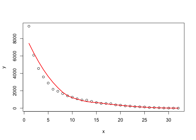
I have 32 months of data, and I'm trying out different models for testing the forecasting of unit transitions to dead state "X" for months 13-32, by training from transitions data for months 1-12. I then compare the forecasts with the actual data for months 13-32. The data represents the unit migration of a beginning population into the dead state over 32 months. Not all beginning units die off, only a portion. I understand that 12 months of data for model training isn't much and that forecasting for 20 months from those 12 months should result in a wide distribution of outcomes, those are the real-world limitations I usually grapple with. I'm working through examples in Hyndman, R.J., & Athanasopoulos, G. (2021) Forecasting: principles and practice , 3rd edition, OTexts: Melbourne, Australia. Forecasting: Principles and Practice (3rd ed) with this data.
When running forecast accuracy tests for the simple forecasting methods described in the text (mean, naive, drift, etc.), for example using accuracy(), CRPS, examining innovation residuals, etc., the "best fit" is the drift method. Note that I get better results when using the ETS model but I use the simple methods for ease of example.
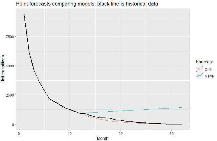
When I run point forecasts per Figure 5.8 of the text for the naive and naive with drift methods using my data, I get the following results:
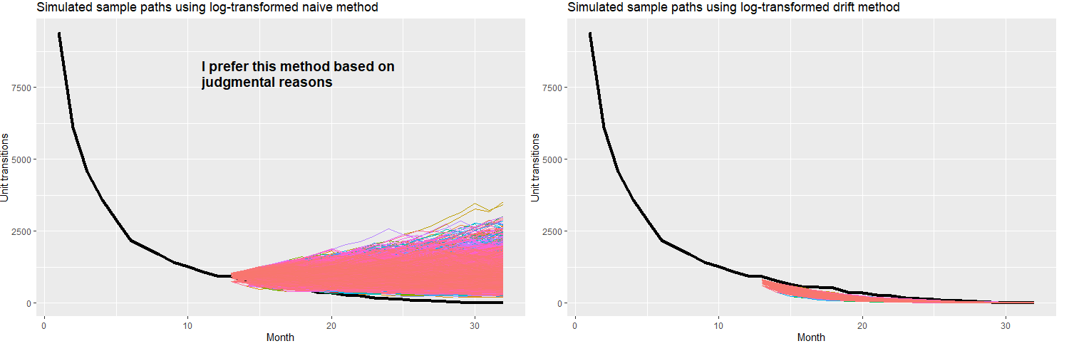
When I run simulation paths for both of these methods per Figure 5.15 of the text I get these results:
I then sum up the forecasted values for both methods for forecast months 13-32 and create histograms, and I also compare the actual data with the mean of the simulation forecasts in the vertical lines as shown below:
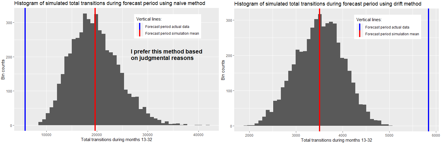
Based on my experience with this type of data, and because in my use of this sort of analysis there is more downside in under-forecasting than in over-forecasting (I need to run MC), my preference is to use the naive method without drift, preferring its wider distribution of outcomes and the fact that it over-forecasts relative to the actual data for forecast period. I would then apply the naive method to other transition curves I come across that share the same general characteristics. Is this sort of judgmental reasoning, overriding in some sense recommendations of model "goodness of fit" tests, considered "statistically robust"? I'm trying to minimize judgment; I'm trying to make this as scientific and objective as possible and am wondering if my thinking is right or wrong in this respect. As an alternative, is there a way to tweak the drift method so that it has a wider distribution of simulated outcomes, and drive it closer to the actual data for the forecast period? Of course, I'm trying to avoid overfitting too.
Here is the code for generating the above, including the data:
library(dplyr)
library(fabletools)
library(fable)
library(feasts)
library(ggplot2)
library(tidyr)
library(tsibble)

DF <- data.frame(
  Month =c(1:32),
  StateX=c(
    9416,6086,4559,3586,2887,2175,1945,1675,1418,1259,1079,940,923,776,638,545,547,510,379,
    341,262,241,168,155,133,76,69,45,17,9,5,0)
  ) %>%
  as_tsibble(index = Month)

### Based on Figure 5.8 ###
train <- DF %>% filter_index(1~12)
fit_models <- train %>%
  model(
    `Naïve` = NAIVE(log(StateX)),
      `Drift` = NAIVE(log(StateX) ~ drift())
  )
fc_models <- fit_models %>% forecast(h = 20)
fc_models %>%
  autoplot(train, level = NULL) +
  autolayer(DF,colour = "black",size = 1.0) +
  labs(
    y = "Unit transitions",
    title = "Point forecasts comparing models: black line is historical data"
  ) +
  guides(colour = guide_legend(title = "Forecast"))

### Based on 5.3 Fitted values and residuals ###
print(as.data.frame(augment(fit_models)))

### Based on Figure 5.15 ###
fitNaive <- DF[1:12,] %>%
  model(NAIVE(log(StateX)))
simNaive <- fitNaive %>% generate(h = 20, times = 5000, bootstrap = TRUE)

DF[1:12,] %>%
  ggplot(aes(x = Month)) +
  autolayer(DF,
    colour = "black", size = 1.5) +
  geom_line(aes(y = StateX)) +
  geom_line(aes(y = .sim, colour = as.factor(.rep)), data = simNaive) +
  labs(title="Simulated sample paths using log-transformed naive method", y="Unit transitions" ) +
  guides(colour = "none")

### Now to generate histogram of simulation using naive method ###
aggSimNaive <- simNaive |>
  as.data.frame() |>
  group_by(.rep) |>
  summarise(sumFC = sum(.sim),.groups = 'drop')

aggSimNaive %>%
  ggplot(aes(x = sumFC)) +
  geom_histogram(bins = 50) +
  geom_vline(
    aes(xintercept = mean(as.data.frame(aggSimNaive)[,"sumFC"]),
        color = "Forecast period simulation mean"),
    linetype="solid",
    size=1.5)+
  geom_vline(
    aes(xintercept = sum(as.data.frame(DF[13:32,"StateX"])),
        color = "Forecast period actual data"
    ),
    linetype="solid", size=1.5) +
  scale_color_manual(
    name = "Vertical lines:",
    values = c(
      'Forecast period actual data' = "blue",
      'Forecast period simulation mean' = "red")) +
  labs(title = "Histogram of simulated total transitions during forecast period using naive method",
       x = 'Total transitions during months 13-32',
       y = 'Bin counts')+
  theme(legend.position = c(0.75,0.85))

### Based on Figure 5.15 ###
fitDrift <- DF[1:12,] %>%
  model(NAIVE(log(StateX)~drift()))
simDrift<- fitDrift %>% generate(h = 20, times = 5000, bootstrap = TRUE)

DF[1:12,] %>%
  ggplot(aes(x = Month)) +
  autolayer(DF,
            colour = "black", size = 1.5) +
  geom_line(aes(y = StateX)) +
  geom_line(aes(y = .sim, colour = as.factor(.rep)), data = simDrift) +
  labs(title="Simulated sample paths using log-transformed drift method", y="Unit transitions" ) +
  guides(colour = "none")

### Now to generate histogram of simulation using drift method ###
simDrift <- fitDrift |>  generate(h = 20, times = 5000, bootstrap = TRUE)

aggSimDrift <- simDrift |>
  as.data.frame() |>
  group_by(.rep) |>
  summarise(sumFC = sum(.sim),.groups = 'drop')

aggSimDrift %>%
  ggplot(aes(x = sumFC)) +
  geom_histogram(bins = 50) +
  geom_vline(
    aes(xintercept = mean(as.data.frame(aggSimDrift)[,"sumFC"]),
        color = "Forecast period simulation mean"),
    linetype="solid", size=1.5) +
  geom_vline(
    aes(xintercept = sum(as.data.frame(DF[13:32,"StateX"])),
        color = "Forecast period actual data"
    ),
    linetype="solid", size=1.5) +
  scale_color_manual(
    name = "Vertical lines:",
    values = c(
      'Forecast period actual data' = "blue",
      'Forecast period simulation mean' = "red"
    )
  ) +
  labs(title = "Histogram of simulated total transitions during forecast period using drift method",
       x = 'Total transitions during months 13-32',
       y = 'Bin counts')+
  theme(legend.position = c(0.75,0.85))
Referred here by Forecasting: Principles and Practice, by Rob J Hyndman and George Athanasopoulos