Example_2 aus_livestock from the Rob J Hyndman book
If the lowest AIC of two methodologies is considered to be the best metthod , I don´t undertand why for this data is showing that ETS (ANA) is a better method than ETS (ANN)?if there is no seasonility why is showing ETS (ANA) a better mehtod than ETS (ANN)
ETS (ANN)
Create variable
library("fpp3")
victoria_pigs <- aus_livestock %>%
  filter(Animal =="Pigs",State == "Victoria") %>%
  view()
Simple exponential smoothing- Error Additive, No trend , No Seasonality
fit <- victoria_pigs%>%
  model(ETS(Count ~ error("A") + trend("N") + season("N")))

fit %>%
report()
Simple exponential smoothing- Error Additive, No trend , Seasonility Additive
fit2 <- victoria_pigs%>%
  model(ETS(Count ~ error("A") + trend("N") + season("A")))

fit2 %>%
report()
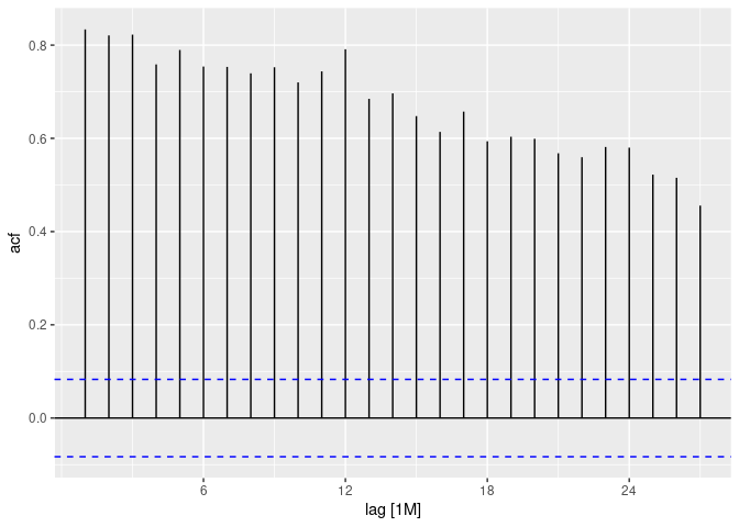
ACF Victorian pigs
victoria_pigs %>%
  ACF(Count, lag_max = 36) %>%
  autoplot()
There are additional tools to gauge seasonality. Also, I wouldn't put too much importance on the small difference between AIC for the two models.
library("fpp3")
#> ── Attaching packages ──────────────────────────────────────────── fpp3 0.4.0 ──
#> ✔ tibble 3.1.8 ✔ tsibble 1.1.1
#> ✔ dplyr 1.0.9 ✔ tsibbledata 0.3.0
#> ✔ tidyr 1.2.0 ✔ feasts 0.2.2
#> ✔ lubridate 1.8.0 ✔ fable 0.3.1
#> ✔ ggplot2 3.3.6
#> ── Conflicts ───────────────────────────────────────────────── fpp3_conflicts ──
#> ✖ lubridate::date() masks base::date()
#> ✖ dplyr::filter() masks stats::filter()
#> ✖ tsibble::intersect() masks base::intersect()
#> ✖ tsibble::interval() masks lubridate::interval()
#> ✖ dplyr::lag() masks stats::lag()
#> ✖ tsibble::setdiff() masks base::setdiff()
#> ✖ tsibble::union() masks base::union()
library(feasts)
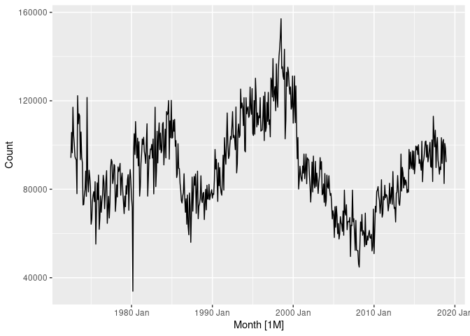
victoria_pigs <- aus_livestock %>%
filter(Animal =="Pigs",State == "Victoria")
autoplot(victoria_pigs)
#> Plot variable not specified, automatically selected `.vars = Count`
victoria_pigs %>% features(Count, feat_stl)
#> # A tibble: 1 × 11
#> Animal State trend…¹ seaso…² seaso…³ seaso…⁴ spiki…⁵ linea…⁶ curva…⁷ stl_e…⁸
#> <fct> <fct> <dbl> <dbl> <dbl> <dbl> <dbl> <dbl> <dbl> <dbl>
#> 1 Pigs Victor… 0.906 0.493 1 7 2.78e10 -46753. -97155. -0.109
#> # … with 1 more variable: stl_e_acf10 <dbl>, and abbreviated variable names
#> # ¹trend_strength, ²seasonal_strength_year, ³seasonal_peak_year,
#> # ⁴seasonal_trough_year, ⁵spikiness, ⁶linearity, ⁷curvature, ⁸stl_e_acf1
#> # ℹ Use `colnames()` to see all variable names
victoria_pigs %>% unitroot_nsdiffs(Count)
#> nsdiffs
#> 0
victoria_pigs %>% features(Count, feat_spectral)
#> # A tibble: 1 × 3
#> Animal State spectral_entropy
#> <fct> <fct> <dbl>
#> 1 Pigs Victoria 0.588
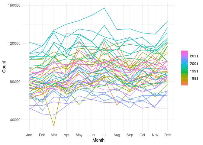
victoria_pigs %>% gg_season(Count)+ theme_minimal()
victoria_pigs %>% ACF(Count) %>% autoplot()
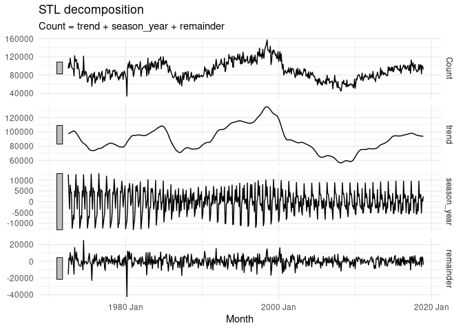
dcmp <- victoria_pigs %>%
model(stl = STL(Count))
components(dcmp)
#> # A dable: 558 x 9 [1M]
#> # Key: Animal, State, .model [1]
#> # : Count = trend + season_year + remainder
#> Animal State .model Month Count trend season_year remainder season…¹
#> <fct> <fct> <chr> <mth> <dbl> <dbl> <dbl> <dbl> <dbl>
#> 1 Pigs Victoria stl 1972 Jul 94200 97261. 12676. -15736. 81524.
#> 2 Pigs Victoria stl 1972 Aug 105700 97844. 4170. 3687. 101530.
#> 3 Pigs Victoria stl 1972 Sep 96500 98426. -3358. 1432. 99858.
#> 4 Pigs Victoria stl 1972 Oct 117100 99009. 7701. 10390. 109399.
#> 5 Pigs Victoria stl 1972 Nov 104600 99509. 4268. 824. 100332.
#> 6 Pigs Victoria stl 1972 Dec 100500 100008. 4247. -3755. 96253.
#> 7 Pigs Victoria stl 1973 Jan 94700 100507. -12361. 6554. 107061.
#> 8 Pigs Victoria stl 1973 Feb 93900 100840. -10139. 3199. 104039.
#> 9 Pigs Victoria stl 1973 Mar 93200 101173. -6261. -1711. 99461.
#> 10 Pigs Victoria stl 1973 Apr 78000 101505. -8123. -15382. 86123.
#> # … with 548 more rows, and abbreviated variable name ¹season_adjust
#> # ℹ Use `print(n = ...)` to see more rows
components(dcmp) %>% autoplot() + theme_minimal()
fit <- victoria_pigs%>%
  model(ETS(Count ~ error("A") + trend("N") + season("N")))

fit %>%
  report()
#> Series: Count
#> Model: ETS(A,N,N)
#>   Smoothing parameters:
#>     alpha = 0.3221247
#>
#>   Initial states:
#>      l[0]
#>  100646.6
#>
#>   sigma^2:  87480760
#>
#>      AIC     AICc      BIC
#> 13737.10 13737.14 13750.07

fit2 <- victoria_pigs%>%
  model(ETS(Count ~ error("A") + trend("N") + season("A")))

fit2 %>%
  report()
#> Series: Count
#> Model: ETS(A,N,A)
#>   Smoothing parameters:
#>     alpha = 0.3579401
#>     gamma = 0.0001000139
#>
#>   Initial states:
#>     l[0]     s[0]    s[-1]     s[-2]     s[-3]     s[-4]     s[-5]   s[-6]
#>  95487.5 2066.235 6717.311 -2809.562 -1341.299 -7750.173 -8483.418 5610.89
#>      s[-7]    s[-8]     s[-9]   s[-10]   s[-11]
#>  -579.8107 1215.464 -2827.091 1739.465 6441.989
#>
#>   sigma^2:  60742898
#>
#>      AIC     AICc      BIC
#> 13545.38 13546.26 13610.24
many thanks!
technocrat:
feat_spectral will compute the (Shannon) spectral entropy of a time series, which is a measure of how easy the series is to forecast. A series which has strong trend and seasonality (and so is easy to forecast) will have entropy close to 0. A series that is very noisy (and so is difficult to forecast) will have entropy close to 1.
that´s fantastic many thanks!
system
October 28, 2022, 2:20pm
6
This topic was automatically closed 7 days after the last reply. New replies are no longer allowed.