How can I generate a GG Diagram in R Studio?

Hello,

I have tried many times, and my R studio doesn't really work out. I have also installed all the packages you guys mentioned, and it comes out like this:-

So I try to run the script on my R Studio, with everything installed except ggplot which is not available for R revision 3.5.1. and it comes out like this "Error in ggplot(acc_1m_and_3m) : could not find function "ggplot""

I have tried the older version of R on R Studio Cloud, ggplot cannot be installed either. Nevertheless, here is my outcome: Posit Cloud

When you installed the packages, this was successful? There were no error messages after the install.packages command(s)?

Are you loading the packages? (that is running library(tidyverse) and library(ggplot2) ) These commands gave you no errors?

I think you need to follow @mara's advice about creating a reprex, as we cannot see what commands you are actually running throughout the session and hence why it might be failing. If you want to pursue this further, this should be your next step. Using the reprex library it should be very easy to do, given that you already have the code you've been running.

I haven't looked at your outcome (I don't use rstudio.cloud) - did you get something to do what you wanted? I hope so. How did you do it? It would be nice to see a reprex of your solution.

3 Likes

Thanks for sharing the project — that should make it easier to understand the problems you are having. However, right now the project can only be accessed by you. To make it viewable by others, click on the gear in the upper right:

28

Then change the Access setting to "Everyone":
48

1 Like

Yes, thanks for notifying me. I hope everyone can access now.

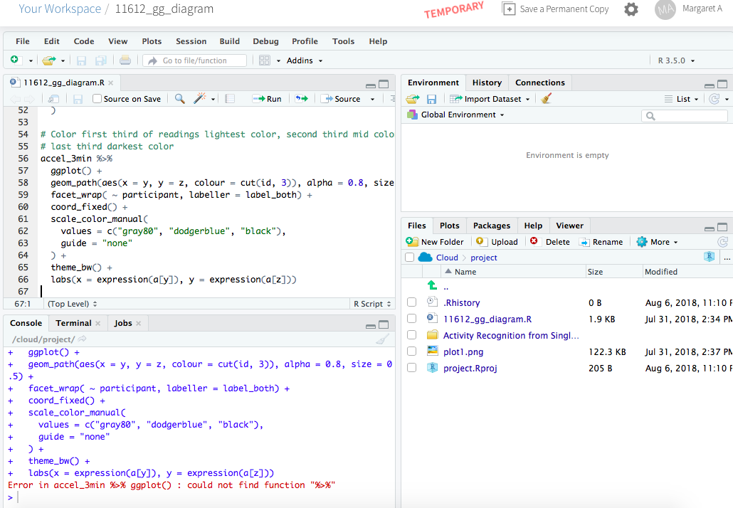
Yes, all the packages were successfully installed. I was using the script provided by you, i.e. the below:-

library(tidyverse)
library(ggplot2)
library(reprex)
#
# Example data file from a X2-2 accelerometer
file_loc <- 'http://www.gcdataconcepts.com/DATA-100.CSV'
#
# Function to load
load_accel <- function(fn, label = NA){
  # Read header lines from the file
  fc <- file(fn)
  hh <- readLines(fc, n = 9)
  close(fc)
  # edit and split the header lines lines
  hhl <- gsub(", ", ",", hh) %>% str_split(",")
  # extract the gain amnd header names
  gain  <- hhl[[grep(";Gain", hhl)]][2]
  heads <- hhl[[grep(";Headers", hhl)]][2:5]
  #
  # Read full data from the file:
  atbl <- read_csv(fn, col_names = heads, comment = ";")
  #
  if( gain == "low" ){ conv_fac <- 1/6554 } else { conv_fac <- 1/13108 }
  atbl %>% mutate( Axg = Ax * conv_fac,
                   Ayg = Ay * conv_fac,
                   Azg = Az * conv_fac, expt =label ) %>%
    # drops expt if all NA, assumes other columns contain values
    select_if(function(x){!all(is.na(x))}) 
}
#
# As you have two experiments/treatments, at 1m and 3m, I've plotted
# the same file twice, once for each. You would have two different file
# locations here.
#
# Assuming you have accelerometer data files at 1m and 3m, this
# code is what you need (with the file names modified to yours):
# acc_1m_and_3m <- bind_rows( load_accel( "my_1m_accel_data.csv", "1m" ),
#                             load_accel( "my_3m_accel_data.csv", "3m" ) )
#
# Because I am re-plotting the same data file twice in this example, I'm
# going to scale the 1m height data to make it less variable:
#
d_1m <- load_accel( file_loc, "1m" ) %>%
  mutate( Axg = Axg*0.5,
          Ayg = Ayg*0.5,
          Azg = Azg*0.5 )
#> Parsed with column specification:
#> cols(
#>   time = col_double(),
#>   Ax = col_integer(),
#>   Ay = col_integer(),
#>   Az = col_integer()
#> )
# and then combine it with the 3m height data:
d_3m <- load_accel( file_loc, "3m" )
#> Parsed with column specification:
#> cols(
#>   time = col_double(),
#>   Ax = col_integer(),
#>   Ay = col_integer(),
#>   Az = col_integer()
#> )
acc_1m_and_3m <- bind_rows( d_1m, d_3m )
#
# Now we're ready to plot the data in acc_1m_and_3m
#
ggplot(acc_1m_and_3m) +
  geom_path(aes(x = Azg, y = Ayg,
                # I'm generating a factor from expt with the levels in
                # a specific order so that the more variable 3m data will
                # be plotted beneath the 1m data, as in the examples
                colour = factor(expt,levels=c("3m","1m"))), size = 0.5) +
  coord_fixed() + theme_bw() +
  scale_x_continuous(name = expression(A[z] (g))) +
  scale_y_continuous(name = expression(A[y] (g))) +
  scale_colour_manual(name = "Height", values=c("dodgerblue","black"))


I am still trying to understand what reprex and how reprex works, it will take me some times to work on it. I will update my reprex outcome here later. Thank you so much.

I'm afraid we're still not quite there yet. You seem to have put this project in its own Workspace. In your screenshot, you can see there is "Your Workspace" and "Tree Data" in the sidebar to the left. In RStudio Cloud, there are two ways of sharing a project:

  • If the project lives inside "Your Workspace", then you can set its access to "Everyone" (like in my screen shot). This effectively makes it public — anybody with the link can access it.
  • If a project lives inside a specific shared Space, then you have to invite people to join that Space and change the project's access to "Everyone in [Space Name]".

So right now, I still can't access your project because I am not a member of your "Tree Data" Space. If you want to share this project with helpers here, it's probably best to move it to "Your Workspace" so you can set its access to "Everyone". You can do that from the main "Tree Data" Space screen (click on Tree Data in the left sidebar, above).

Thanks so much for your detailed explanation. I have created a new sample here - https://rstudio.cloud/project/54521

Thank you so much for everyone's help again.

1 Like