Applying UK Post Codes values to UK regions

Hi,
I have this sample df with scores and UK post codes:

region.scores <- data.frame(
  stringsAsFactors = FALSE,
                               Shop = c("A","B","C","D","E","F","G",
                                         "H","I","J","K","L","M","N","O",
                                         "P","Q","R","S","T","U","V",
                                         "W","X","Y","Z"),
                            GoogleSc = c(4,4.5,4.2,4.2,3.6,4.5,4.3,
                                         4.7,4.3,4.3,4.4,4.6,4.5,4.2,4.4,
                                         4.2,3.9,4,3.9,4.3,3.7,4.5,4.6,
                                         4.4,3.5,4.1),
                        FullPostCode = c("AB16 6HQ","GU12 4NY","HP19 8DP",
                                         "OX16 3TL","LL57 4YH","EX32 8QA",
                                         "SS14 3EQ","BA2 3AY","BT3 9JP",
                                         "B7 5EA","BL3 6HH","BH12 3LL","CF31 3SA",
                                         "BN3 7ES","BS2 0HL","BB11 5UB",
                                         "BL9 7AZ","CT1 2RJ","CF23 9AB","CA2 7AF",
                                         "CM1 2GL","CH1 4NT","S41 8JT",
                                         "CV6 4BQ","RH10 9PG","CR0 4XN"),
                            PostCode = c("AB16","GU12","HP19","OX16",
                                         "LL57","EX32","SS14","BA2","BT3",
                                         "B7","BL3","BH12","CF31","BN3","BS2",
                                         "BB11","BL9","CT1","CF23","CA2",
                                         "CM1","CH1","S41","CV6","RH10",
                                         "CR0"),
                                Cor1 = c(57.161,51.251,51.822,52.062,
                                         53.207,51.071,51.575,51.36,54.62,
                                         52.493,53.565,50.737,51.509,50.835,
                                         51.46,53.783,53.592,51.277,51.515,
                                         54.884,51.745,53.202,53.247,52.432,
                                         51.117,51.372),
                                Cor2 = c(-2.156,-0.731,-0.825,-1.34,
                                         -4.111,-4.018,0.476,-2.377,-5.904,
                                         -1.873,-2.431,-1.926,-3.576,-0.174,
                                         -2.581,-2.252,-2.286,1.087,-3.151,
                                         -2.949,0.457,-2.908,-1.427,-1.507,
                                         -0.157,-0.074),
                     PostCode2digits = c("AB","GU","HP","OX","LL","EX",
                                         "SS","BA","BT","B7","BL","BH",
                                         "CF","BN","BS","BB","BL","CT","CF",
                                         "CA","CM","CH","S4","CV","RH",
                                         "CR"),
                              Region = c("Scotland","South East",
                                         "East of England","South East","Wales",
                                         "South West","East of England",
                                         "South West","Northern Ireland","West Midlands",
                                         "North West","South West","Wales",
                                         "South East","South West","North West",
                                         "North West","South East","Wales",
                                         "North West","East of England",
                                         "North West","Yorkshire and the Humber",
                                         "West Midlands","South East",
                                         "Greater London"),
                                City = c("Aberdeen","Guilford",
                                         "Hemel Hempstead","Oxford","Llandudno",
                                         "Exeter","Southend on Sea","Bath",
                                         "Northern Ireland","Birmingham","Bolton",
                                         "Bournemouth","Cardiff","Brighton",
                                         "Bristol","Blackburn","Bolton",
                                         "Canterbury","Cardiff","Carlisle","Chelmsford",
                                         "Chester","Sheffield","Coventry",
                                         "Redhill","Croydon")
                  )


region.scores

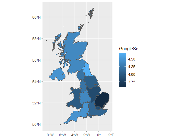
I can prepare UK map for Google scores using this code:

library(tidyverse)
library(sf)

uk.all <- left_join(uk, region.scores, by = c('name'='PostCode'))
uk.all
uk.all %>% filter(!is.na(GoogleSc))

rs_sf <- st_as_sf(region.scores, coords=c('Cor2','Cor1'), crs=st_crs(uk.all))

GoogleSc.UK <- ggplot()+
  geom_sf(data=uk.all,mapping=aes(fill=GoogleSc)) +
  scale_fill_gradient(low = "#F8766D", high = "#00BA38") +
  labs(title = "Google Scores by region",
       fill = "Google Score") 

GoogleSc.UK 

The maps are almost empty.
Is it possible to apply the score to Region to have the entire UK map coloured?

what is the source of this ? your code is not reproducible without it

Sorry, I forgot about this part:

#Download UK postcode polygon Shapefile

download.file(
  "http://www.opendoorlogistics.com/wp-content/uploads/Data/UK-postcode-boundaries-Jan-2015.zip",
  "postal_shapefile"
)
unzip("postal_shapefile")

uk <- read_sf('Distribution/Districts.shp')

you dont seem to have the requisite parts; i..e. region boundaries; or the postcode to region memberships for the unscored postcodes.

you might be able to do something complex like find the closest coloured polygon to any given uncoloured polygon and assign colour from that; but I don't think I have the time to experiment with that; perhaps someone that works more with maps than I do will have code for that sort of thing.

Can we simply somehow use existing "Region" variable?

Scores.by.region <- region.scores %>%
  group_by(Region) %>%
  summarise_at(.vars = vars(ends_with(match = "GoogleSc")),.funs = list(Sc = ~mean(.,na.rm=TRUE), Count = ~sum(!is.na(.))))
Scores.by.region

We just need to link scores with "Regions" but I don't know how

from this code you have 'East of England 4.07', you will need to download a map that has polygon for East of England, and use that; or else the map you have which is of postcodes; you would need to know what postcodes are in East of England to give them all 4.07.

Can I use this instead?

library(tidyverse)
library(rnaturalearth)
library(readxl)

library(rgeos)
germany <- ne_states(country = "germany", returnclass = "sf") %>%
  select(name)

url_regions <- "https://biogeo.ucdavis.edu/data/gadm3.6/Rsf/gadm36_DEU_3_sf.rds"

scored_regions <- readRDS(url(url_regions)) %>% 
  filter(NAME_1 %in% region.scores$NAME_1) %>% 
  full_join(region.scores)

I just need to change Germany into UK somehow but I don't know how :frowning:

uk <- ne_states(country = 'united kingdom', returnclass = "sf") %>%
  select(name)

I have updated my code to:

library(tidyverse)
library(rnaturalearth)

region.scores <- data.frame(
  stringsAsFactors = FALSE,
  NAME_1 = c("East Midlands",
             "East of England","Greater London","North East","North West",
             "Northern Ireland","Scotland","South East","South West",
             "Wales","West Midlands","Yorkshire and the Humber",
             "Grand Total"),
  GoogleSc = c(3.86,3.56363636363636,
               3.86666666666667,4.7,4.21111111111111,4.475,4.38571428571429,
               4.09444444444444,4.46470588235294,4,4.37777777777778,
               4.03333333333333,4.15773195876289)
)

library(rgeos)
uk <- ne_states(country = 'united kingdom', returnclass = "sf") %>%
  select(name)

# You can download this file from the GDAM site
url_regions <- "https://biogeo.ucdavis.edu/data/gadm3.6/Rsf/gadm36_DEU_3_sf.rds"

scored_regions <- readRDS(url(url_regions)) %>% 
  filter(NAME_1 %in% region.scores$NAME_1) %>% 
  full_join(region.scores)

head(scored_regions)

ggplot() +
  geom_sf(data = uk, alpha = 0.3) +
  geom_sf(data = scored_regions, aes(fill = GoogleSc)) +
  scale_fill_gradient(low = "red", high = "green") +
  labs(title = "Dealer Rec Score by region",
       fill = "Scores") +
  theme_minimal() +
  theme(plot.title = element_text(hjust = 0.5, size = 20),
        axis.title = element_blank(),
        plot.background = element_blank(),
        legend.position = c(0.95, 0.20),
        plot.margin = margin(5, 0, 5, 0))

but it is not working.
I think I need to change this:

url_regions <- "https://biogeo.ucdavis.edu/data/gadm3.6/Rsf/gadm36_DEU_3_sf.rds"

to the UK version?

I think I found a way (almost). I can create this map:


library(rgdal)
eng <- rgdal::readOGR(paste0("https://opendata.arcgis.com/datasets/",
                             "8d3a9e6e7bd445e2bdcc26cdf007eac7_4.geojson"))

countries <- rgdal::readOGR(paste0("https://opendata.arcgis.com/datasets/",
                                   "92ebeaf3caa8458ea467ec164baeefa4_0.geojson"))

eng <- sf::st_as_sf(eng)
countries <- sf::st_as_sf(countries)
UK <- countries[-1,] 
names(eng)[3] <- "Region"
names(UK)[3] <- "Region"
UK$objectid <- 10:12
eng <- eng[-2]
UK <- UK[c(1, 3, 9:11)]
UK <- rbind(eng, UK)

ggplot2::ggplot(UK, ggplot2::aes(fill = Region)) + ggplot2::geom_sf()

But the map generates random scores.
I have my own scores:

region.scores <- data.frame(
  stringsAsFactors = FALSE,
  Region= c("East Midlands",
             "East of England","London","North East","North West",
             "Northern Ireland","Scotland","South East","South West",
             "Wales","West Midlands","Yorkshire and the Humber",
             "Grand Total"),
  GoogleSc = c(3.86,3.56363636363636,
               3.86666666666667,4.7,4.21111111111111,4.475,4.38571428571429,
               4.09444444444444,4.46470588235294,4,4.37777777777778,
               4.03333333333333,4.15773195876289)
)
region.scores

How can I apply these scores to the map?
How can I change colouring from red to green? I cannot find scale_fill_gradient in the code.

I also have this solution:


#Clear the memory
rm(list=ls())
#Download some important packages
library(maps)
library(mapdata)
library(maptools)
library(rgdal)
library(ggmap)
library(ggplot2)
library(rgeos)
library(broom)
library(plyr)

#Load the shapefile - make sure you change the filepath to where you saved the shapefiles
shapefile <- readOGR(dsn="C:/Users/SDanilowicz/OneDrive - MARQUE GROUP HOLDINGS PTY LTD/GeoInfo/UK/NUTS_Level_1_(January_2018)_Boundaries", layer="NUTS_Level_1_(January_2018)_Boundaries")

#Reshape for ggplot2 using the Broom package
mapdata <- tidy(shapefile, region="nuts118nm") #This might take a few minutes
mapdata

#Check the shapefile has loaded correctly by plotting an outline map of the UK
gg <- ggplot() + geom_polygon(data = mapdata, aes(x = long, y = lat, group = group), color = "#FFFFFF", size = 0.25)
gg <- gg + coord_fixed(1) #This gives the map a 1:1 aspect ratio to prevent the map from appearing squashed
print(gg)

region.scores <- data.frame(
  stringsAsFactors = FALSE,
  id = c("East Midlands (England)",
         "East of England","London","North East (England)","North West (England)",
         "Northern Ireland","Scotland","South East (England)","South West (England)",
         "Wales","West Midlands (England)","Yorkshire and the Humber"),
  value = c(3.86,3.56363636363636,
            3.86666666666667,4.7,4.21111111111111,4.475,4.38571428571429,
            4.09444444444444,4.46470588235294,4,4.37777777777778,
            4.03333333333333)
)
region.scores

#Join mydata with mapdata
df <- join(mapdata, region.scores, by="id")

#Create the heatmap using the ggplot2 package
gg <- ggplot() + geom_polygon(data = df, aes(x = long, y = lat, group = group, fill = value), color = "#FFFFFF", size = 0.25)
gg <- gg + scale_fill_gradient2(low = "red", mid = "yellow", high = "green", na.value = "white")
gg <- gg + coord_fixed(1)
gg <- gg + theme_minimal()
gg <- gg + theme(panel.grid.major = element_blank(), panel.grid.minor = element_blank(), legend.position = 'none')
gg <- gg + theme(axis.title.x=element_blank(), axis.text.x = element_blank(), axis.ticks.x = element_blank())
gg <- gg + theme(axis.title.y=element_blank(), axis.text.y = element_blank(), axis.ticks.y = element_blank())
print(gg)

but the map is green with one missing region (not missing?)
What do you think?

Anyone? I can see I am on my own with this...

I can only ignore the most recent proposal as it include private data from your one drive.
You were quite close with the previous attempt


library(rgdal)
eng1 <- rgdal::readOGR(paste0("https://opendata.arcgis.com/datasets/",
                             "8d3a9e6e7bd445e2bdcc26cdf007eac7_4.geojson"))

countries1 <- rgdal::readOGR(paste0("https://opendata.arcgis.com/datasets/",
                                   "92ebeaf3caa8458ea467ec164baeefa4_0.geojson"))

eng <- sf::st_as_sf(eng1)
countries <- sf::st_as_sf(countries1)
UK <- countries[-1,] 
names(eng)[3] <- "Region"
names(UK)[3] <- "Region"
UK$objectid <- 10:12
eng <- eng[-2]
UK <- UK[c(1, 3, 9:11)]
UK <- rbind(eng, UK)


region.scores <- data.frame(
  stringsAsFactors = FALSE,
  Region= c("East Midlands",
            "East of England","London","North East","North West",
            "Northern Ireland","Scotland","South East","South West",
            "Wales","West Midlands","Yorkshire and The Humber", # uppercase `The`
            "Grand Total"),
  GoogleSc = c(3.86,3.56363636363636,
               3.86666666666667,4.7,4.21111111111111,4.475,4.38571428571429,
               4.09444444444444,4.46470588235294,4,4.37777777777778,
               4.03333333333333,4.15773195876289)
)

ukj <- left_join(UK,region.scores)

ggplot2::ggplot(ukj, ggplot2::aes(fill = GoogleSc)) + ggplot2::geom_sf()

image

Thank you!
Can you help me to change colours (red to green) please?

use

 + scale_fill_gradient(low="#FF0000", high = "#00FF00")

the colours are hex codes for RGB so alter as you wish

1 Like

This topic was automatically closed 7 days after the last reply. New replies are no longer allowed.

If you have a query related to it or one of the replies, start a new topic and refer back with a link.