Exponential regression

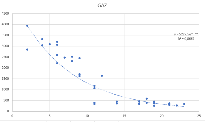
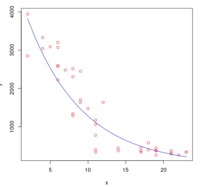
I want to do an exponential regression with this data in order to compare with linear and polynomial model.
TEMPERATURE;GAZ
8;1290
8;1340
10;1474
11;777
18;397
22;263
21;370
18;578
14;444
7;2478
6;3201
4;3330
8;2518
8;2306
12;1635
14;369
17;458
21;315
23;336
19;442
11;1062
9;2450
5;3088
2;3945
6;3070
6;2594
9;1705
11;398
19;369
19;261
19;379
17;371
11;339
6;2219
4;3044
2;2850
6;2584
9;1630
11;1174
17;337
21;293
23;337

My results for the linear model :
Call:
lm(formula = GAZ ~ TEMPERATURE, data = edf)

Residuals:
Min 1Q Median 3Q Max
-1251.29 -278.31 84.01 364.99 919.76

Coefficients:
Estimate Std. Error t value Pr(>|t|)
(Intercept) 3344.1 183.3 18.25 < 2e-16 ***
TEMPERATURE -159.4 13.4 -11.90 1.02e-14 ***

Signif. codes: 0 β€˜β€™ 0.001 β€˜β€™ 0.01 β€˜β€™ 0.05 β€˜.’ 0.1 β€˜ ’ 1

Residual standard error: 538.7 on 40 degrees of freedom
Multiple R-squared: 0.7797, Adjusted R-squared: 0.7742
F-statistic: 141.6 on 1 and 40 DF, p-value: 1.021e-14
My results for the polynomial model :
lm(formula = GAZ ~ TEMPERATURE + I(TEMPERATURE^2), data = edf)

Residuals:
Min 1Q Median 3Q Max
-1026.93 -82.48 40.43 135.98 798.55

Coefficients:
Estimate Std. Error t value Pr(>|t|)
(Intercept) 4706.316 279.455 16.841 < 2e-16 ***
TEMPERATURE -436.194 50.380 -8.658 1.28e-10 ***
I(TEMPERATURE^2) 10.752 1.917 5.607 1.82e-06 ***

Signif. codes: 0 β€˜β€™ 0.001 β€˜β€™ 0.01 β€˜β€™ 0.05 β€˜.’ 0.1 β€˜ ’ 1

Residual standard error: 406 on 39 degrees of freedom
Multiple R-squared: 0.878, Adjusted R-squared: 0.8718
F-statistic: 140.4 on 2 and 39 DF, p-value: < 2.2e-16
GRAPHIQUE.pdf (8.4 KB)

If you are asking how to do exponential regression in R....
I did a google search 'exponential regression in R' and got you this lesson
Exponential Regression in R (Step-by-Step) - Statology

But, with this answer, i can't have directly the expression of the exponential curve and the tests. I want to have this expression
Capture d’écran 2022-08-11 232717

Isnt the equation of the curve there in your image, above R squared.

I want to have the equation and the R-Squared with R.

Use coef() function to extract the coefficients of your model

Things like r2 can be extracted from the summary() of your model with code like
summary(model)$r.squared

Yes, but, i donc know to do the exponential model. I want to learn to make this non-linear regression.
The plot in the topic comes from Excel

You should seek an appropriate tutorial.
This forum is ideal for addressing concrete problems, or answer concise questions as they arise during a course of work.

From my perspective its overoptimistic to expect to get a wholistic education in a substantial topic - directly on this forum.

Concretly, my code is this
model <- nls(CHAUFFAGE ~ a * exp(-b * THIVER),
data = hiver,
start = list(a = 1, b = 1))
But, the Console shows this error
Error in numericDeriv(form[[3L]], names(ind), env, central = nDcentral) :
Valeur manquante ou infinie obtenue au cours du calcul du modèle

Try setting a and b closer to the values found in Excel.

To expand on starts, try following the code from this stack overflow thread: Exponential regression with nls in R - Stack Overflow

You should fit a simple log model first to get better starting points for a and b and specify an algorithm. Your error is also in french so I'm not sure what it refers to, but the following code is your solution (in regards to the code).

df = structure(list(x = c(8, 8, 10, 11, 18, 22, 21, 18, 14, 7, 6, 
4, 8, 8, 12, 14, 17, 21, 23, 19, 11, 9, 5, 2, 6, 6, 9, 11, 19, 
19, 19, 17, 11, 6, 4, 2, 6, 9, 11, 17, 21, 23), y = c(1290, 1340, 
1474, 777, 397, 263, 370, 578, 444, 2478, 3201, 3330, 2518, 2306, 
1635, 369, 458, 315, 336, 442, 1062, 2450, 3088, 3945, 3070, 
2594, 1705, 398, 369, 261, 379, 371, 339, 2219, 3044, 2850, 2584, 
1630, 1174, 337, 293, 337)), class = c("tbl_df", "tbl", "data.frame"
), row.names = c(NA, -42L))

o <- order(df$x)
df_o <- df[o, ] # order it by increasing x

fm0 <- lm(log(y) ~ I(-x), df_o) # simpler model to get better starting values

st <- list(b = coef(fm0)[[2]])
fm <- nls(y ~ cbind(a = exp(-b*x)), df_o, start = st, alg = "plinear")

plot(df_o, col = "red", pch = 20)
lines(fitted(fm) ~ x, df_o)

summary(fm)  #coefficients to create the equation
1 Like

Does not agree with your Excel answer, but is this closer to what you are looking for?

y = a*(b^x)

LNy = LN[a*(b^x)] = LNa + LN(b^x) = LNa + xLNb

The above is a linear equation in x.

The resulting linear regression gives intercept parameter LNa and slope parameter LNb

e^(LNy) = e[1] = e[2] * e[3] = a * e^LN[b^x]

y = a * b^x, where a = e^(intercept parameter), and b = e^(slope parameter)

x = c(8, 8, 10, 11, 18, 22, 21, 18, 14, 7, 6,
4, 8, 8, 12, 14, 17, 21, 23, 19, 11, 9, 5, 2, 6, 6, 9, 11, 19,
19, 19, 17, 11, 6, 4, 2, 6, 9, 11, 17, 21, 23)
y = c(1290, 1340,
1474, 777, 397, 263, 370, 578, 444, 2478, 3201, 3330, 2518, 2306,
1635, 369, 458, 315, 336, 442, 1062, 2450, 3088, 3945, 3070,
2594, 1705, 398, 369, 261, 379, 371, 339, 2219, 3044, 2850, 2584,
1630, 1174, 337, 293, 337)

model <- lm(log(y) ~ x)
intercept <- model$coefficients[1]
slope <- model$coefficients[2]
a <- exp(intercept)
b <- exp(slope)
print( paste("y = ", round(a,4), "*", round(b,4), "^x"))

plot(x, y, col = "red")
curve(a * b^x, col= "blue", add = TRUE)

[1] "y = 5034.3697 * 0.8718 ^x"


  1. LNa + xLNb β†©οΈŽ

  2. LNa β†©οΈŽ

  3. xLNb β†©οΈŽ

@fcas80 is showing you the easy way to do it. Taking logs gets you to a linear regression.

You should know though that you won't get exactly the same results if you do it this way (@fcas80 points out that the results are different) because the error terms are handled differently when you take logs or when you don't.

1 Like

This topic was automatically closed 21 days after the last reply. New replies are no longer allowed.

If you have a query related to it or one of the replies, start a new topic and refer back with a link.