Issue:
I have been struggling with rescaling the loadings (arrows) length in a ggplot2/ggbiplot in a PCA biplot. I have researched extensively through StackOverflow, on the web, and I've asked the R Studio Community to resolve my issue, although, the only information that I can find is either through different biplot functions or a reference to other entirely different packages for PCA (MASS, factoextra, FactoMineR, PCAtools, and many others), none of which address the question that I would like to answer.
What am I missing? I would really like to continue using ggbiplot/ggplot2 to get a better understanding of both packages and I prefer the visual representation of the output plot in diagram 1 (see R code 1 below)
So far, my most successful attempt to rescale the loadings (arrows) was using the function geom_segment() and geom_label() (see R-code 2 and diagram 2). The problem is the new arrows have overlayed themselves on top of the original arrows from diagram 1 (there are now short and long loadings in diagram 2: 16 arrows for 8 parameters), and the labels with grey backgrounds are now in the foreground and have not adjusted to the right position at the end of arrowheads.
Desired plot
Ideally, I would like the biplot to resemble diagram 3 (see below) where the loadings (arrows) are longer and just slightly thicker (like diagram 2) and the labels with grey backgrounds are not overlapping each other (like diagram 3) and sit neatly at the end of the loading arrowheads. I used the argument varname.adjust()for the labels in diagram 1 but I'm not sure how to apply this to the functions geom_segment() and geom_label() in diagram 2.
If anyone can help, I would be deeply appreciative.
Many thanks in advance
Dummy Data
#Dummy data
#Create a cluster column with dummy data (clusters = 3)

f1 <- gl(n = 2, k=167.5); f1

#Produce a data frame for the dummy level data
f2<-as.data.frame(f1)

#Rename the column f2
colnames(f2)<-"Country"

#How many rows
nrow(f2)

#Rename the levels of the dependent variable 'Country' as classifiers
#prefer the inputs to be factors
levels(f2$Country) <- c("France", "Germany")

#Create random numbers
Start.Freq<-runif(335, min=1.195110e+02, max=23306.000000)
End.Freq<-runif(335, min=3.750000e+02, max=65310.000000)
Delta.Time<-runif(335, min=2.192504e-02, max=3.155762)
Low.Freq<-runif(335, min=6.592500e+02, max=20491.803000)
High.Freq<-runif(335, min=2.051000e+03, max=36388.450000)
Peak.Freq<-runif(335, min=7.324220+02, max=35595.703000)
Center.Freq<-runif(335, min=2.190000e-02, max=3.155800)
Delta.Freq<-runif(335, min=1.171875+03, max=30761.719000)
Delta.Time<-runif(335, min=2.192504e-02, max=3.155762)

#Bind the columns together
Bind<-cbind(f2, Start.Freq, End.Freq,  Low.Freq, High.Freq, Peak.Freq,  Center.Freq, Delta.Freq, Delta.Time)

#Rename the columms
colnames(Bind)<-c('Country', 'Low.Freq', 'High.Freq', 'Start.Freq', 'End.Freq', 'Peak.Freq', 'Center.Freq',
                  'Delta.Freq', 'Delta.Time')

#Produce a dataframe
Whistle_Parameters<-as.data.frame(Bind)
Whistle_Parameters
Data Transformation
#Open library packages
library(MASS)
library(car)

#Create a dataframe format for the Yeo transform
Box<-as.data.frame(Whistle_Parameters)
Box

#Check the structure of the dataframe 'Box'
str(Box)

#Use the function powerTransform(), specifying family = "bcPower", to obtain an optimal Box Cox transformation
transform_Low.Freq.box=car::powerTransform(Box$Low.Freq, family= "bcPower")
transform_Low.Freq.box

transform_High.Freq.box=car::powerTransform(Box$High.Freq, family= "bcPower")
transform_High.Freq.box

transform_Start.Freq.box=car::powerTransform(Box$Start.Freq, family= "bcPower")
transform_Start.Freq.box

transform_End.Freq.box=car::powerTransform(Box$End.Freq, family= "bcPower")
transform_End.Freq.box

transform_Peak.Freq.box=car::powerTransform(Box$Peak.Freq, family= "bcPower")
transform_Peak.Freq.box

transform_Center.Freq.box=car::powerTransform(Box$Center.Freq, family= "bcPower")
transform_Center.Freq.box

transform_Delta.Freq.box=car::powerTransform(Box$Delta.Freq, family= "bcPower")
transform_Delta.Freq.box

transform_Delta.Time.box=car::powerTransform(Box$Delta.Time, family= "bcPower")
transform_Delta.Time.box

#save transformed Box Cox data in strand_box to compare both
stand_box=Box
stand_box[,5]=bcPower(Box[,5],transform_Low.Freq.box$lambda)
stand_box[,6]=bcPower(Box[,6],transform_High.Freq.box$lambda)
stand_box[,7]=bcPower(Box[,7],transform_Start.Freq.box$lambda)
stand_box[,8]=bcPower(Box[,8],transform_End.Freq.box$lambda)
stand_box[,9]=bcPower(Box[,9],transform_Peak.Freq.box$lambda)
stand_box[,10]=bcPower(Box[,10],transform_Center.Freq.box$lambda)
stand_box[,11]=bcPower(Box[,11],transform_Delta.Freq.box$lambda)
stand_box[,12]=bcPower(Box[,12],transform_Delta.Time.box$lambda)

#Check the structure of the new stand_box Yeo-Johnson transformed data
str(stand_box)

#Produce a dataframe object
Box_Cox_Transformation<-as.data.frame(stand_box)
Box_Cox_Transformation

#Check the structure of the new stand_trans Yeo-Johnson transformed data
str(Box_Cox_Transformation)
R-code 1
install.packages("remotes")
remotes::install_github("vqv/ggbiplot")
install_github("vqv/ggbiplot")

#install.packages("devtools")
library(devtools)
library(ggbiplot)
library(remotes)

#You can do a PCA to visualize the difference between the groups using the standardised box cox data
PCA=prcomp(Whistle_Parameters[2:18], center = TRUE, scale=TRUE, retx = T)

#PCA biplot
PCA_plot<-ggbiplot(PCA, ellipse=TRUE, circle=TRUE, varname.adjust = 2.5, groups=Box_Cox_Stan_Dataframe$Country, var.scale = 1) +
                  ggtitle("PCA of Acoustic Parameters") +
                  theme(plot.title = element_text(hjust = 0.5)) +
                  theme_minimal() +
                  theme(panel.background = element_blank(),
                  panel.grid.major = element_blank(),
                  panel.grid.minor = element_blank(),
                  panel.border = element_blank()) +
                  theme(axis.line.x = element_line(color="black", size = 0.8),
                  axis.line.y = element_line(color="black", size = 0.8))

#Place the arrows in the forefront of the points
PCA_plot$layers <- c(PCA_plot$layers, PCA_plot$layers[[2]])

#The options for styling the plot within the function itself are somewhat limited, but since it produces a
#ggplot object, we can re-specify the necessary layers. The following code should work on any object
#output from ggbiplot. First we find the geom segment and geom text layers:

seg <- which(sapply(PCA_plot$layers, function(x) class(x$geom)[1] == 'GeomSegment'))
txt <- which(sapply(PCA_plot$layers, function(x) class(x$geom)[1] == 'GeomText'))

#We can change the colour and width of the segments by doing
PCA_plot$layers[[seg[1]]]$aes_params$colour <- 'black'
PCA_plot$layers[[seg[2]]]$aes_params$colour <- 'black'

#Labels
# Extract loadings of the variables
PCAloadings <- data.frame(Variables = rownames(PCA$rotation), PCA$rotation)

#To change the labels to have a gray background, we need to overwrite the geom_text layer with a geom_label layer:
  PCA_plot$layers[[txt]] <- geom_label(aes(x = xvar, y = yvar, label = PCAloadings$Variables,
                                       angle = 0.45, hjust = 0.5, fontface = "bold"),
                                       label.size = NA,
                                       data = PCA_plot$layers[[txt]]$data,
                                       fill = '#dddddd80')

  PCA_plot
R-code 2
#Labels
# Extract loadings of the variables
PCAloadings <- data.frame(Variables = rownames(PCA$rotation), PCA$rotation)

#PCA biplots
PCA_plot1<-ggbiplot(PCA, ellipse=TRUE, circle=TRUE, varname.adjust = 2.5, groups=Box_Cox_Stan_Dataframe$Country, var.scale = 1) +
                   ggtitle("PCA of Acoustic Parameters") +
                   theme(plot.title = element_text(hjust = 0.5)) +
                   theme_minimal() +
                   theme(panel.background = element_blank(),
                   panel.grid.major = element_blank(),
                   panel.grid.minor = element_blank(),
                   panel.border = element_blank()) +
                   theme(axis.line.x = element_line(color="black", size = 0.8),
                   axis.line.y = element_line(color="black", size = 0.8)) +
                   geom_segment(data = PCAloadings, aes(x = 0, y = 0, xend = (PC1*4.6),
                                yend = (PC2*4.6)), arrow = arrow(length = unit(1/2, "picas")),
                                color = "black")

#Place the arrows in the forefront of the points
PCA_plot1$layers <- c(PCA_plot1$layers, PCA_plot1$layers[[2]])

#The options for styling the plot within the function itself are somewhat limited, but since it produces a
#ggplot object, we can re-specify the necessary layers. The following code should work on any object
#output from ggbiplot. First we find the geom segment and geom text layers:
seg <- which(sapply(PCA_plot1$layers, function(x) class(x$geom)[1] == 'GeomSegment'))
txt <- which(sapply(PCA_plot1$layers, function(x) class(x$geom)[1] == 'GeomText'))

#We can change the colour and width of the segments by doing
PCA_plot1$layers[[seg[1]]]$aes_params$colour <- 'black'
PCA_plot1$layers[[seg[2]]]$aes_params$colour <- 'black'

#To change the labels to have a gray background, we need to overwrite the geom_text layer with a geom_label layer:
PCA_plot1$layers[[txt]] <- geom_label(aes(x = xvar, y = yvar, label = PCAloadings$Variables,
                                         angle = 0.45, hjust = 0.5, fontface = "bold"),
                                         label.size = NA,
                                         data = PCA_plot1$layers[[txt]]$data,
                                         fill = '#dddddd80')
PCA_plot1
Diagram 1
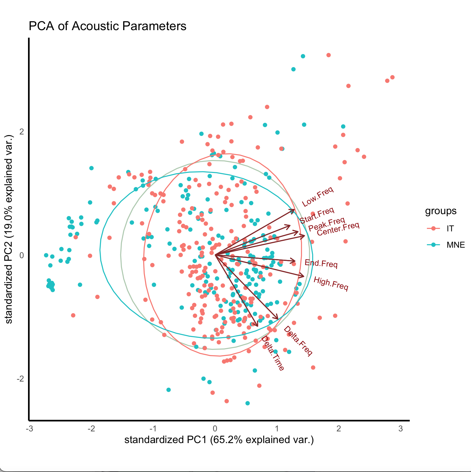
Diagram 2 - These arrows overlay the original arrows in diagram 1 and are positioned incorrectly
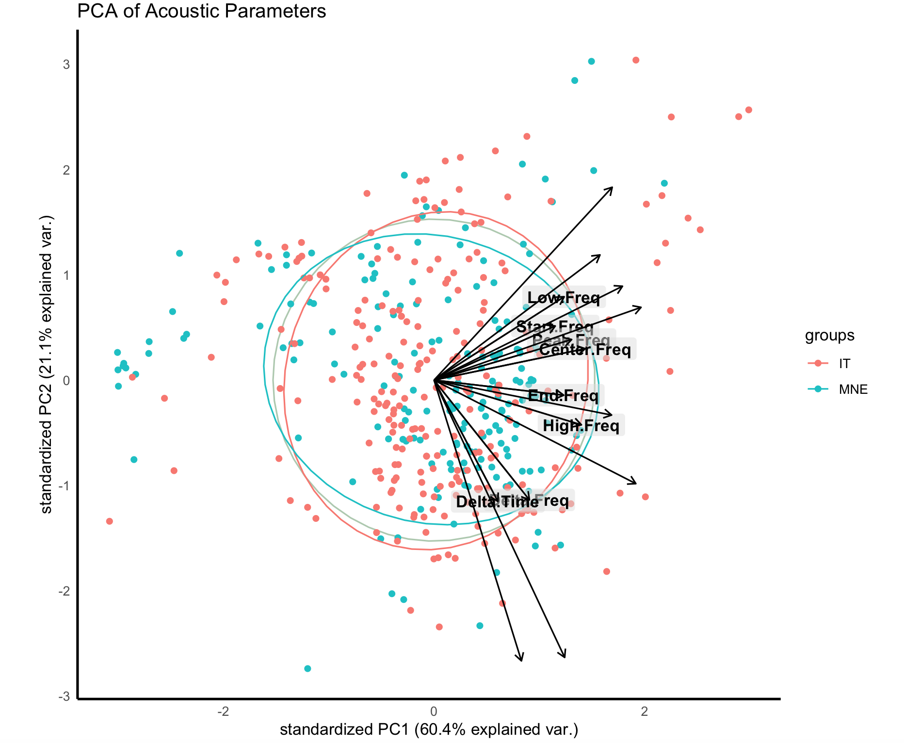
Diagram 3 - Desired Output
