How can I perform multiple linear models by accumulating the groups

[kmilovelez]

I have a database with stable isotope measurements: deuterium and oxygen_18.
Both variables have been quantified monthly (there are some NAs per month) in rainwater from 2005 to 2014. In this case, the year is a group or a factor. I am trying to perform a lineal regression lm(deuterium ~ oxygen_18) by group (by year) but in such a way that the first model run the first group (2005), the second model analyzes the first and the second group (2005 and 2006), the third model run the first, the second and third groups (2005, 2006 and 2007) and so on until the latest model includes all the data from 2005 to 2014.

So far I have been able to perform the regression by group:

model.year <- df %>%
  nest(data = -Year) %>% 
  mutate(
    fit = map(
      data,
      ~ lm(Deuterio ~ Oxigeno, data = .x)
      ),
    tidied = map(fit, tidy)
  ) %>% 
  unnest(tidied)

Any suggestions as to how I could do this?

[startz]

Something like

for (iYear in 2005:2014){
 partial_df <- df |> filter(Year<=iYear)
 lm(Deuterio ~ Oxigeno, data = partial_df)
}

[technocrat]

The how part is straightforward, the what part needs closer examination.

# data
d <- data.frame(year = c(
  2005, 2005, 2005, 2005, 2005, 2005,
  2005, 2005, 2005, 2005, 2005, 2005, 2006, 2006, 2006,
  2006, 2006, 2006, 2006, 2006, 2006, 2006, 2006, 2006,
  2007, 2007, 2007, 2007, 2007, 2007, 2007, 2007, 2007,
  2007, 2007, 2007, 2008, 2008, 2008, 2008, 2008, 2008,
  2008, 2008, 2008, 2008, 2008, 2008, 2009, 2009, 2009,
  2009, 2009, 2009, 2009, 2009, 2009, 2009, 2009, 2009,
  2010, 2010, 2010, 2010, 2010, 2010, 2010, 2010, 2010,
  2010, 2010, 2010, 2011, 2011, 2011, 2011, 2011, 2011,
  2011, 2011, 2011, 2011, 2011, 2011, 2012, 2012, 2012,
  2012, 2012, 2012, 2012, 2012, 2012, 2012, 2012, 2012,
  2013, 2013, 2013, 2013, 2013, 2013, 2013, 2013, 2013,
  2013, 2013, 2013, 2014, 2014, 2014, 2014, 2014, 2014,
  2014, 2014, 2014, 2014, 2014, 2014
), month = c(
  1, 2, 3,
  4, 5, 6, 7, 8, 9, 10, 11, 12, 1, 2, 3, 4, 5, 6, 7, 8, 9, 10,
  11, 12, 1, 2, 3, 4, 5, 6, 7, 8, 9, 10, 11, 12, 1, 2, 3, 4, 5,
  6, 7, 8, 9, 10, 11, 12, 1, 2, 3, 4, 5, 6, 7, 8, 9, 10, 11, 12,
  1, 2, 3, 4, 5, 6, 7, 8, 9, 10, 11, 12, 1, 2, 3, 4, 5, 6, 7, 8,
  9, 10, 11, 12, 1, 2, 3, 4, 5, 6, 7, 8, 9, 10, 11, 12, 1, 2, 3,
  4, 5, 6, 7, 8, 9, 10, 11, 12, 1, 2, 3, 4, 5, 6, 7, 8, 9, 10,
  11, 12
), h2 = c(
  1, 1, 65, 1, 1, 54, 20, 1, 0, 1, 22, 38, 1, 2,
  0, 1, 3, 29, 1, 1, 0, 55, 1, 3, 63, 1, 0, 4, 1, 4, 6, 2, 1, 0,
  1, 1, 1, 2, 1, 3, 1, 1, 0, 3, 13, 49, 1, 2, 8, 3, 8, 4, 0, 0,
  1, 1, 3, 1, 2, 0, 45, 1, 2, 13, 0, 1, 1, 1, 65, 49, 65, 63, 1,
  8, 5, 20, 3, 52, 49, 1, 4, 1, 6, 1, 0, 72, 2, 1, 6, 1, 1, 94,
  3, 3, 4, 49, 1, 1, 4, 1, 4, 0, 0, 0, 0, 2, 65, 3, 3, 1, 1, 78,
  2, 0, 2, 1, 1, 1, 5, 1
), o18 = c(
  55, 1, 25, 88, 65, 33, 1, 15,
  11, 47, 23, 55, 1, 24, 31, 94, 23, 16, 78, 70, 33, 25, 99, 53,
  71, 6, 1, 23, 25, 54, 71, 94, 73, 23, 97, 88, 14, 4, 91, 94,
  25, 35, 40, 40, 25, 33, 47, 12, 23, 14, 33, 55, 55, 12, 40, 22,
  31, 88, 36, 75, 55, 47, 46, 41, 31, 33, 34, 94, 97, 31, 14, 23,
  18, 33, 16, 6, 16, 47, 34, 18, 47, 12, 47, 18, 33, 15, 77, 40,
  49, 1, 75, 1, 51, 45, 94, 18, 12, 73, 33, 45, 23, 11, 35, 73,
  71, 33, 47, 41, 41, 71, 35, 85, 16, 12, 31, 27, 39, 78, 49, 94
))

my_lm <- function(x) lm(h2 ~ o18,d[unlist(groups[x]),])

groups <- split(1:120,ceiling(seq_along(1:120) / 12))

# examine the last group, for example

my_lm(10) |> summary()
#> 
#> Call:
#> lm(formula = h2 ~ o18, data = d[unlist(groups[x]), ])
#> 
#> Residuals:
#>     Min      1Q  Median      3Q     Max 
#> -22.596  -6.603  -2.540   1.229  57.466 
#> 
#> Coefficients:
#>             Estimate Std. Error t value Pr(>|t|)
#> (Intercept)  -8.3904    12.6671  -0.662    0.523
#> o18           0.3403     0.2309   1.474    0.171
#> 
#> Residual standard error: 20.99 on 10 degrees of freedom
#> Multiple R-squared:  0.1784, Adjusted R-squared:  0.09623 
#> F-statistic: 2.171 on 1 and 10 DF,  p-value: 0.1714

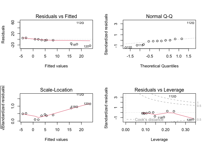
# show diagnostics

par(mfrow = c(2, 2))
plot(my_lm(10))

# use time series linear regression

library(fpp3)
#> ── Attaching packages ────────────────────────────────────────────── fpp3 0.5 ──
#> ✔ tibble      3.2.1     ✔ tsibble     1.1.3
#> ✔ dplyr       1.1.1     ✔ tsibbledata 0.4.1
#> ✔ tidyr       1.3.0     ✔ feasts      0.3.1
#> ✔ lubridate   1.9.2     ✔ fable       0.3.3
#> ✔ ggplot2     3.4.1     ✔ fabletools  0.3.2
#> ── Conflicts ───────────────────────────────────────────────── fpp3_conflicts ──
#> ✖ lubridate::date()    masks base::date()
#> ✖ dplyr::filter()      masks stats::filter()
#> ✖ tsibble::intersect() masks base::intersect()
#> ✖ tsibble::interval()  masks lubridate::interval()
#> ✖ dplyr::lag()         masks stats::lag()
#> ✖ tsibble::setdiff()   masks base::setdiff()
#> ✖ tsibble::union()     masks base::union()

# convert to time series in tsibble format

dts <- as_tsibble(ts(d[3:4], start = c(2005,1), frequency = 12))
dts <- dts |> pivot_wider(names_from = key)

dts |>
  model(TSLM(h2 ~ o18)) |>
  report()
#> Series: h2 
#> Model: TSLM 
#> 
#> Residuals:
#>     Min      1Q  Median      3Q     Max 
#> -13.897 -10.909  -8.484  -4.985  80.103 
#> 
#> Coefficients:
#>             Estimate Std. Error t value Pr(>|t|)    
#> (Intercept) 13.95972    3.57794   3.902 0.000159 ***
#> o18         -0.06263    0.07244  -0.865 0.388981    
#> ---
#> Signif. codes:  0 '***' 0.001 '**' 0.01 '*' 0.05 '.' 0.1 ' ' 1
#> 
#> Residual standard error: 21.38 on 118 degrees of freedom
#> Multiple R-squared: 0.006296,    Adjusted R-squared: -0.002125
#> F-statistic: 0.7476 on 1 and 118 DF, p-value: 0.38898

^{Created on 2023-03-30 with reprex v2.0.2}