HOW to add exponential trend line on RStudio ? To show bacterial growth curve for example

[marlexis]

Hello, I'm new up there ! I'm not very good in Rstudio so please be patient lol (and i'm french so non native english speaker)

I'm in master's degree internship and I have collected data of bacteria concentration (cell/ml) above time (in days of experiment). So My supervisor wants me to plot the abundance above time and to add exponential trendline (with equation of the trendline and Rsquare). As simple as it is on Excel, i would like to do it on R, but I NEVER SUCCEDED and I went on so many website. I don't understand why this seems so complicated. I really need help because my internship end soon, so please if someone succeed to help me, I would appreciate.
Someone on stack overflow told me to just copy the curve given by excel, but I'm sure there is a way to calculate it with Rstudio.

Also on Excel, you can choose to trace the tendance curve on just some point of the data but still plot all the point (idk if this is clear but), for example let's imagine I know from what I see when I plot my data, that there is an exponential growth from the day 1 to day 6, and after it "calm down" and decrease. So I just want the exponential trendline to be calculated from the day 1 to 6. is it possible on R ??

Please, I beg someone to help me ..

here are an example of my data
C2A <- data.frame(cell = c(7.0710000,
5.2810000,
5.4210000,
5.5810000,
1.26100000,
1.121000000,
1.551000000,
2.501000000,
3.34*1000000),
day = c(0,3,4,5,7,11,12,13,14))

[startz]

How about

library(tidyverse)
C2AShort <- C2A |> filter(day <= 6)
reg <- lm(log(cell)~day, data = C2AShort)
summary(reg)

[marlexis]

Hello and thanks,
is "| >" a language from tidyverse package , because with this symbol >, the console say this :
Error: unexpected '>' in "C2AShort <- C2A |>"

I tried to install of course tidyverse.... but it struggle a lot. Btw this is another problem but I have problem installing some packages sometimes. Stuff about binary version, and it looked trought many internet link to download the package.

[nirgrahamuk]

@startz

|>

This is the R pipe, introduce in Version 4.1.0 in May 2021
To use it you would need to upgrade R itself.
if you have magrittr/dplyr/tidyverse packages you could use that instead,
load them and use %>% which is the version they provided before R itself gave us |>

for problems with installation, its somewhat platform dependant. What Operating System do you use ?

[startz]

"|>" is the pipe symbol. It is only available in the more recent versions of R. It is not part of tidyverse. You can write

C2AShort <- filter( C2A, day <= 6)

instead.
(Ninjaed by @nirgrahamuk )

[nirgrahamuk]

it seems that lm doesnt give good symetric results for log(y)~x compared to y~exp(x)

library(tidyverse)
C2A <- data.frame(
  cell = c(
    7.0710000,
    5.2810000,
    5.4210000,
    5.5810000,
    1.26100000,
    1.121000000,
    1.551000000,
    2.501000000,
    3.34 * 1000000
  ),
  day = c(0, 3, 4, 5, 7, 11, 12, 13, 14)
)

(day1plus <- C2A |> filter(day >= 1))

# doesnt look great
ggplot(data = C2A) +
  aes(x = day, y = cell) +
  geom_point() +
  geom_smooth(
    data = day1plus,
    method = "lm", formula = log(y) ~ x
  )
![image|557x408](upload://i0XWP8Gye4XaRtpNohxKMJIogRz.png)

# looks better  ? 
ggplot(data = C2A) +
  aes(x = day, y = cell) +
  geom_point() +
  geom_smooth(
    data = day1plus,
    method = "lm", formula = y ~ exp(x)
  )
![image|557x408](upload://e7ZuejLRmxeVyTSttidwDoHZHnG.png)



(mylm_1 <- lm(formula = log(cell) ~ day,data=day1plus))
summary(mylm_1)

(mylm_2 <- lm(formula = cell ~ exp(day),data=day1plus))
summary(mylm_2)

[EconProf]

The exponential growth function is y = Ae^bx, where A is the y-intercept and b is the growth rate. The formula y ~ exp(x) would estimate y = a + be^x instead

The exponential function can be estimated by taking the log of both sides, resulting in log(y) = a + bx where a = log(A), hence the formula log(y) ~ x

[marlexis]

My R version is : RStudio 2023.03.0 "Cherry Blossom". I have a Macbook air (sorry lol) on 13.0.1.

[marlexis]

Okay thanks and once I got the summary result, Which parameter should I use to plot my exponential trendline ?

[startz]

summary(reg) gives

Coefficients:
            Estimate Std. Error t value Pr(>|t|)   
(Intercept)  1.91580    0.08207  23.343  0.00183 **
day         -0.05278    0.02321  -2.274  0.15084   

So your plot is cell = exp(-0.05 + 0.02*day). But do give some thought to the comments by @nirgrahamuk and @econprof about the best functional form.

[marlexis]

Hello, thanks for your answer. On excel, the equation with exponential trendline is well y=Ae^bx and not y = a + be^x

[EconProf]

Because a = log(A), then A = e^a so y = (A)(e^bx ) = (e^a)(e^bx) = e^(a + bx)

library(tidyverse)

C2A <- data.frame(cell = c(7.071,
                           5.281,
                           5.421,
                           5.581,
                           1.261,
                           1.121,
                           1.551,
                           2.501,
                           3.341),
                  day = c(0,3,4,5,7,11,12,13,14))

# limit regression to days 0, 3, 4 and 5
# use a log-linear model to estimate an exponential function

C2AShort <- C2A |> filter(day <= 6)
reg <- C2AShort |> lm(formula = log(cell) ~ day)
summary(reg)
#> 
#> Call:
#> lm(formula = log(cell) ~ day, data = C2AShort)
#> 
#> Residuals:
#>        1        2        3        4 
#>  0.04021 -0.09333 -0.01438  0.06750 
#> 
#> Coefficients:
#>             Estimate Std. Error t value Pr(>|t|)   
#> (Intercept)  1.91580    0.08207  23.343  0.00183 **
#> day         -0.05278    0.02321  -2.274  0.15084   
#> ---
#> Signif. codes:  0 '***' 0.001 '**' 0.01 '*' 0.05 '.' 0.1 ' ' 1
#> 
#> Residual standard error: 0.08686 on 2 degrees of freedom
#> Multiple R-squared:  0.7211, Adjusted R-squared:  0.5816 
#> F-statistic:  5.17 on 1 and 2 DF,  p-value: 0.1508

# Plot line segments using fitted values from the regression model
# I also plotted all the data points

C2A |> 
  mutate(fit_exp = exp(1.91580 - 0.0528 * day)) |> 
  ggplot(aes(day, fit_exp)) + 
  geom_line() +
  geom_point(aes(y = cell))

# mutate(fit_exp = exp(1.91580) * exp(-0.0528 * day)) also works

^{Created on 2023-04-13 with reprex v2.0.2}

[marlexis]

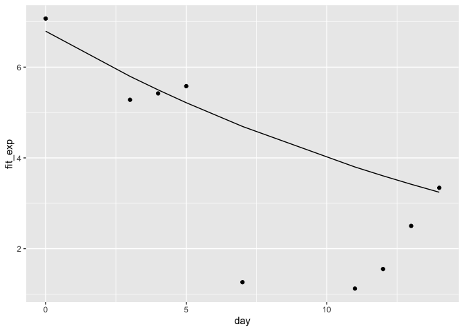
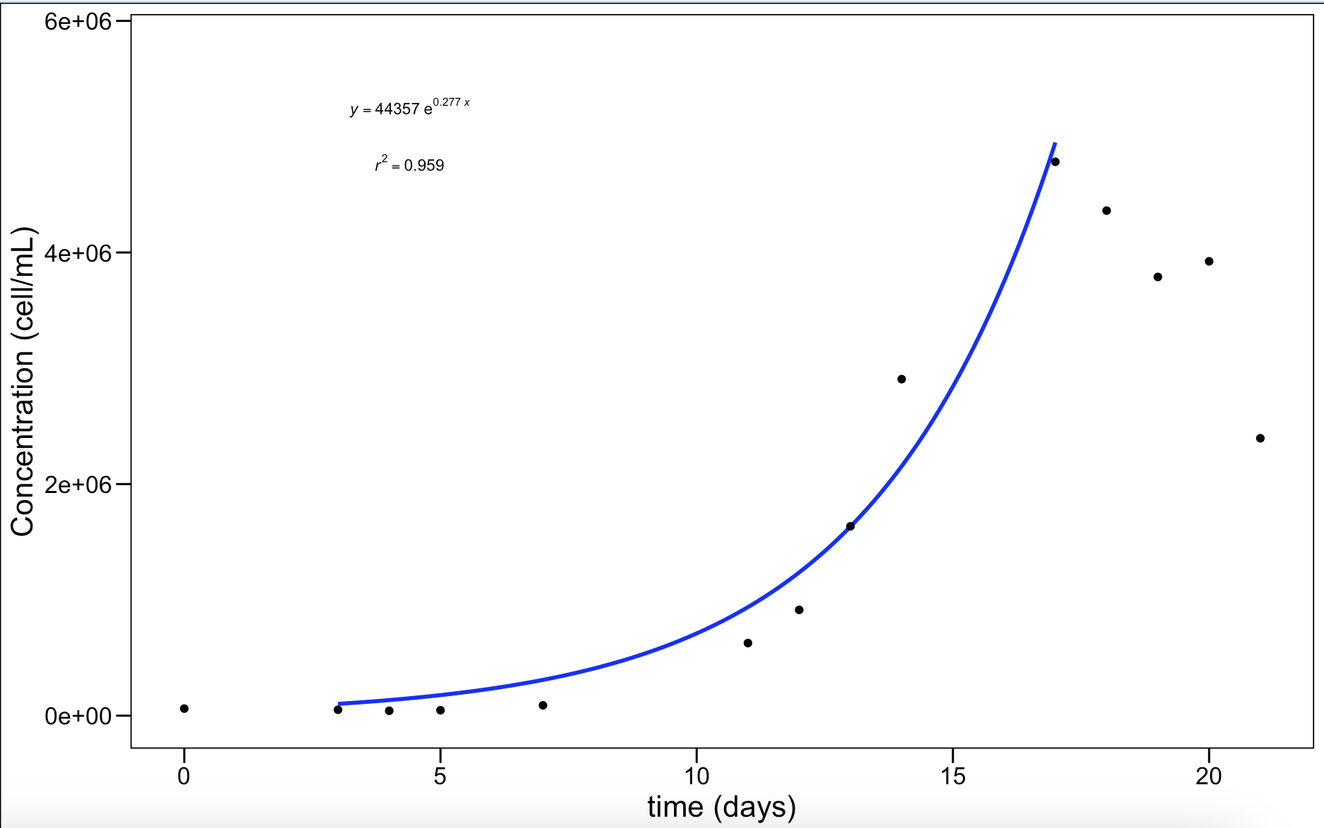
Hi to you all, okay I've found a solution
I'm using ggtrendline package which gave me good results . I wrote the script but I don't know I did it well, don't understand how we are supposed to add code line.

So this method looks great !

BUT NOW, sorry to bother you all, but I would like to merge 3 graphs like this in one (I have 3 plot from my 3 replicate) and I would like to plot them in one. It seems like this package ggtrendline does not allow this.

I've tried 2 solutions :

• to run the same code for my 3 replicate, and to put the three graphs in ONE PAGE and I didn't succeed
• or to use the package on my dataframe regrouping the three replicate.

thanks a lot and have great day

C2Bt <- read.csv("C2B.csv",sep = ";")
timeB <- c(3,4,5,7,11,12,13,14,17)
abundanceB <- c(5.10*10000,
                4.24*10000,
                4.69*10000,
                8.91*10000,
                6.27*100000,
                9.14*100000,
                1.64*1000000,
                2.91*1000000,
                4.78*1000000)

ggtrendline(timeB, abundanceB, model = "exp2P", linecolor = "blue", linetype = 1, 
            linewidth = 1,show.pvalue = FALSE, CI.fill = NA,CI.alpha=0,CI.color = "white")+
  geom_point(data = C2Bt, aes(x = Days_C2B, y = Concentration_C2B)) + 
  theme_base() + labs (x="time (days)", y="Concentration (cell/mL)")

``