How to calculate area under the disease progress stairs. I have the following code, what could be the issue?

[BlackEinstein]

ibrary(agricolae)
dates<-c(7,14,21,28,35,42,49) # days

example 1: evaluation - vector

evaluation<-c(16.5,22.82,22.86,41.23, 47.90, 52.62, 56.49)
audps(evaluation,dates)
audps(evaluation,dates,"relative")
x<-seq(15.5,60.5,7)
y<-c(40,80,90,90)
plot(x,y,"s",ylim=c(0,100),xlim=c(16,62),axes=FALSE,col="red" ,ylab="",xlab="")
title(cex.main=0.8,main="Absolute or Relative AUDPS\nTotal area=(31.5-10.5)*100=2100",
ylab="evaluation",xlab="dates" )
points(x,y,type="h")
z<-c(14,21,28)
points(z,y[-3],col="blue",lty=2,pch=19)
points(z,y[-3],col="blue",lty=2,pch=19)
axis(1,x,pos=0)
axis(2,c(0,40,80,90,100),las=2)
text(dates,evaluation+5,dates,col="blue")
text(14,20,"A = (17.5-10.5)*40",cex=0.8)
text(21,40,"B = (24.5-17.5)*80",cex=0.8)
text(28,60,"C = (31.5-24.5)*90",cex=0.8)
text(14,95,"audps = A+B+C = 1470")
text(14,90,"relative = audps/area = 0.7")

It calculates audpc absolute

absolute<-audps(evaluation,dates,type="absolute")
print(absolute)
rm(evaluation, dates, absolute)

[technocrat]

@BlackEinstein

plot(x,y,"s",ylim=c(0,100),xlim=c(16,62),axes=FALSE,col="red" ,ylab="",xlab="")

Let's start here. x and y differ in length()

Error in xy.coords(x, y, xlabel, ylabel, log) : 
  'x' and 'y' lengths differ
> x
[1] 15.5 22.5 29.5 36.5 43.5 50.5 57.5
> y
[1] 40 80 90 90

Compare the example, where dates and evaluation are of equal length

library(agricolae)
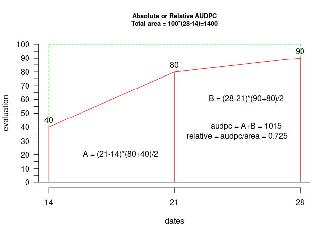
dates <- c(14, 21, 28) # days
# example 1: evaluation - vector
evaluation <- c(40, 80, 90)
audpc(evaluation, dates)
#> evaluation 
#>       1015
# example 2: evaluation: dataframe nrow=1
evaluation <- data.frame(E1 = 40, E2 = 80, E3 = 90) # percentages
plot(dates, evaluation, type = "h", ylim = c(0, 100), col = "red", axes = FALSE)
title(cex.main = 0.8, main = "Absolute or Relative AUDPC\nTotal area = 100*(28-14)=1400")
lines(dates, evaluation, col = "red")
text(dates, evaluation + 5, evaluation)
text(18, 20, "A = (21-14)*(80+40)/2")
text(25, 60, "B = (28-21)*(90+80)/2")
text(25, 40, "audpc = A+B = 1015")
text(24.5, 33, "relative = audpc/area = 0.725")
abline(h = 0)
axis(1, dates)
axis(2, seq(0, 100, 5), las = 2)
lines(rbind(c(14, 40), c(14, 100)), lty = 8, col = "green")
lines(rbind(c(14, 100), c(28, 100)), lty = 8, col = "green")
lines(rbind(c(28, 90), c(28, 100)), lty = 8, col = "green")

# It calculates audpc absolute
absolute <- audpc(evaluation, dates, type = "absolute")
print(absolute)
#> [1] 1015
rm(evaluation, dates, absolute)
# example 3: evaluation dataframe nrow>1
data(disease)
dates <- c(1, 2, 3) # week
evaluation <- disease[, c(4, 5, 6)]
# It calculates audpc relative
index <- audpc(evaluation, dates, type = "relative")
# Correlation between the yield and audpc
correlation(disease$yield, index, method = "kendall")
#> 
#> Kendall's rank correlation tau
#> 
#> data: disease$yield and index 
#> z-norm =  -3.326938 p-value = 0.0008780595 
#> alternative hypothesis: true rho is not equal to 0
#> sample estimates:
#> tau
#>  -0.5436832
# example 4: days infile
data(CIC)
comas <- CIC$comas
oxapampa <- CIC$oxapampa
dcomas <- names(comas)[9:16]
days <- as.numeric(substr(dcomas, 2, 3))
AUDPC <- audpc(comas[, 9:16], days)
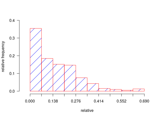
relative <- audpc(comas[, 9:16], days, type = "relative")
h1 <- graph.freq(AUDPC, border = "red", density = 4, col = "blue")

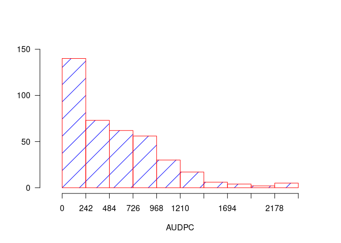
table.freq(h1)
h2 <- graph.freq(relative,
  border = "red", density = 4, col = "blue",
  frequency = 2, ylab = "relative frequency"
)

^{Created on 2022-11-22 by the reprex package (v2.0.1)}