How to use geom text or geom_label position in facets/panels with different scales?

[Tavo_Cera]

Hi Rstudio Community,

The example below is a dummy version (with mtcars data) of the plot I want to create. At the end you will find a reprex and the output generated.

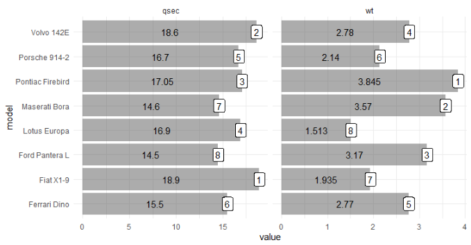
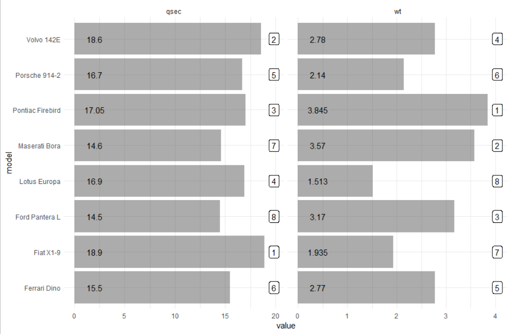
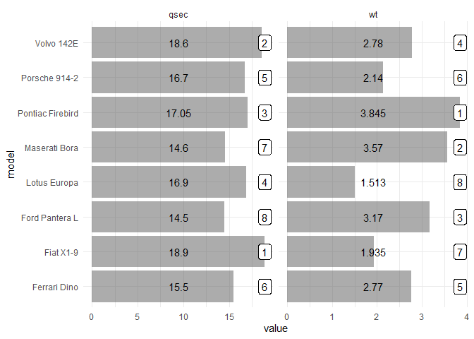
I want to plot two metrics with geom_col and facet_wrap. Each bar represents an observation (in this case a car model) and each facet/panel a different metric. I pretend to extend this plot to more than two metrics. There are two labels to plot for each bar: the metric value and the rank position.

I want to use geom_label to visualize the ranking value and I want to locate it at the far right of each facet. That means, I want the rank number at the top of the highest value and display every car ranking in that position.

However, I haven't been able to locate the ranking in a consistent position for every bar. Arguments like hjust or nudge_x depends on each bar value and even the position functions an its paddings haven't work out for me. The facets having different scale adds a level of complexity because the maximum values are very different.

Is there a way to solve this: locating a label in a consistent position for every facet no matter the scale?
If not, how should I visualize both metric values and metric ranks in order to separate/differentiate between them and make it as easier as possible for the reader to identify them?

Thanks in advance, here is the code:

library(dplyr)
library(tidyr)
library(ggplot2)

mtcars %>% 
  as_tibble(rownames = "model") %>% 
  select(model, wt, qsec) %>% 
  tail(8) %>% 
  pivot_longer(-model, names_to = "metric", values_to = "value") %>% 
  group_by(metric) %>% 
  mutate(rank = dense_rank(-value)) %>% 
  ungroup() %>% 
  ggplot() + 
  aes(value, model) + 
  geom_col(alpha = .5) + 
  geom_text(aes(x = value * .5, label = value)) + 
  geom_label(aes(label = rank)) + 
  facet_wrap(~metric, scales = "free_x") + 
  theme_minimal()

[nirgrahamuk]

library(tidyverse)

mydata <- mtcars %>% 
  as_tibble(rownames = "model") %>% 
  select(model, wt, qsec) %>% 
  tail(8) %>% 
  pivot_longer(-model, names_to = "metric", values_to = "value") %>% 
  group_by(metric) %>% 
  mutate(rank = dense_rank(-value),
         maxval=max(value)*1.05) %>% 
  ungroup() 

mydata %>% 
  ggplot() + 
  aes(value, model) + 
  geom_col(alpha = .5) + 
  geom_text(aes(x=maxval/10,label = value)) + 
  geom_label(aes(x = maxval,label = rank)) + 
  facet_wrap(~metric, scales = "free_x") + 
  theme_minimal()

[FJCC]

I might have misunderstood your goal. Is this what you want?

library(tidyverse)
mtcars %>% 
  as_tibble(rownames = "model") %>% 
  select(model, wt, qsec) %>% 
  tail(8) %>% 
  pivot_longer(-model, names_to = "metric", values_to = "value") %>% 
  group_by(metric) %>% 
  mutate(rank = dense_rank(-value),
         Top = max(value)) %>% 
  ungroup() %>% 
  ggplot() + 
  aes(value, model) + 
  geom_col(alpha = .5) + 
  geom_text(aes(x = Top * .5, label = value)) + 
  geom_label(aes(label = rank,x=Top)) + 
  facet_wrap(~metric, scales = "free_x") + 
  theme_minimal()

^{Created on 2022-11-03 with reprex v2.0.2}

[Tavo_Cera]

This is excellent, thanks both @nirgrahamuk and @FJCC for the answers.
The max value calculation is the last piece I wanted and I was missing.
I'll pick @nirgrahamuk answer as the solution as you responded earlier and the extra .05 after the max is nicer.
Thank you both!