LHS continuous and RHS continuous is not problematic so long as the diagnostics get proper attention and overfitting is avoided.
LHS continuous and RHS binary had the awkward situation of a regression curve that has an intercept and slope for only the beginning and end, with nothing in between, as there is no Schrödinger’s binary provided for or a quantum regression methodology to go with it.
LHS binary and RHS continuous is an issue discussed recently here with one view being that it should never be used over logistic regression and the other that so long as R^2 is ignored ordinary least squares may be used.
LHS binary and R binary under logit regression
summary(fit5 <- glm(vs ~ am, data = mtcars, family = binomial(link = logit)))
#>
#> Call:
#> glm(formula = vs ~ am, family = binomial(link = logit), data = mtcars)
#>
#> Deviance Residuals:
#>     Min       1Q   Median       3Q      Max
#> -1.2435  -0.9587  -0.9587   1.1127   1.4132
#>
#> Coefficients:
#>             Estimate Std. Error z value Pr(>|z|)
#> (Intercept)  -0.5390     0.4756  -1.133    0.257
#> am            0.6931     0.7319   0.947    0.344
#>
#> (Dispersion parameter for binomial family taken to be 1)
#>
#>     Null deviance: 43.860  on 31  degrees of freedom
#> Residual deviance: 42.953  on 30  degrees of freedom
#> AIC: 46.953
#>
#> Number of Fisher Scoring iterations: 4
par(mfrow = c(2,2))
plot(fit5)
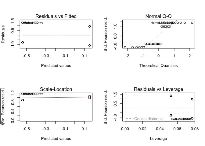
appears to have the same diagnostic plot issues as the lm() example. Should different diagnostics be used? Is it simply the arbitrary selection of variables? Insufficient data? Are non-parametric required?