Hi folks,
I was trying to produce a .Rmd template to use for generating an html report of my RNAseq analyses.
This output should include a data frame with the results (rendered with the command DT::datatable) followed by a set of plots related to that data frame.
An example of my .Rmd code is:
title: ""
author: "r paste0('GeneTonic happy_hour (v', utils::packageVersion('GeneTonic'), ')')"
date: "r Sys.Date()"
output:
html_document:
toc: true
toc_float: true
code_folding: hide
code_download: false
number_sections: true
df_print: kable
theme: lumen
always_allow_html: yes
knitr::opts_chunk$set(
  echo = TRUE,
  warning = FALSE,
  message = FALSE,
  error = TRUE
)
# knitr::opts_knit$set(
#   progress = FALSE,
#   verbose = FALSE
# )
rm(list=ls())
library(GeneTonic)
library("macrophage")
library("DESeq2")
library("org.Hs.eg.db")
library("AnnotationDbi")
Preparing the required data:
# dds object
data("gse", package = "macrophage")
dds_macrophage <- DESeqDataSet(gse, design = ~ line + condition)
rownames(dds_macrophage) <- substr(rownames(dds_macrophage), 1, 15)
dds_macrophage <- estimateSizeFactors(dds_macrophage)

vst_data <- vst(dds_macrophage)

# annotation object
anno_df <- data.frame(
  gene_id = rownames(dds_macrophage),
  gene_name = mapIds(org.Hs.eg.db,
                     keys = rownames(dds_macrophage),
                     column = "SYMBOL",
                     keytype = "ENSEMBL"
  ),
  stringsAsFactors = FALSE,
  row.names = rownames(dds_macrophage)
)


# res object
data(res_de_macrophage, package = "GeneTonic")
res_de <- res_macrophage_IFNg_vs_naive

# res_enrich object
data(res_enrich_macrophage, package = "GeneTonic")
res_enrich <- shake_topGOtableResult(topgoDE_macrophage_IFNg_vs_naive)
res_enrich <- get_aggrscores(res_enrich, res_de, anno_df)

# gtl list:
gtl <- GeneTonicList(
  dds = dds_macrophage,
  res_de = res_de,
  res_enrich = res_enrich,
  annotation_obj = anno_df
)
Plotting the data:
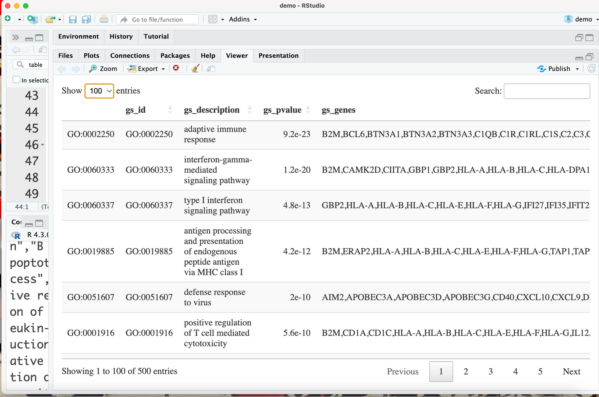
cat(" \nDataframe of the results is here:")
print(htmltools::tagList(DT::datatable(res_enrich)))
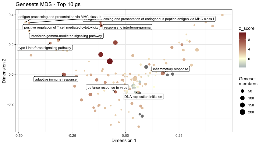
#### ~~~ MDS: ~~~ ####
cat(" \n**Geneset MDS plot**: A Multi Dimensional Scaling plot for gene sets. Color coded by the *[z-score](http://www.bioconductor.org/packages/release/bioc/vignettes/GeneTonic/inst/doc/GeneTonic_manual.html#2_Getting_started)* (a score attempts to determine the “direction” of change")
print(gs_mds(gtl = gtl,
mds_colorby = 'z_score',
mds_labels = 10,
plot_title = "Genesets MDS - Top 10 gs"))
#### ~~~ENRICHMENT MAP: ~~~ ####
cat(" \n**Enrichment map**: An interactive plot which shows the relationship between genesets (more info [here](https://journals.plos.org/plosone/article?id=10.1371/journal.pone.0013984)). Genesets are dots and the segment that connect genesets indicate shared genes between genesets.
Only the first 50 gene sets are included in the plot, and are color-coded by their p-value. \n")
em <- enrichment_map(gtl = gtl,
n_gs = 50,
overlap_threshold = 0.1,
scale_edges_width = 200,
color_by = 'gs_pvalue',
scale_nodes_size = 5,
)
library("igraph")
library("visNetwork")
library("magrittr")
print(htmltools::tagList(em %>% # To print this, see this post https://stackoverflow.com/questions/60685631/using-ggplotly-and-dt-from-a-for-loop-in-rmarkdown
visIgraph() %>%
visOptions(highlightNearest = list(enabled = TRUE,
degree = 1,
hover = TRUE),
nodesIdSelection = TRUE) %>%
visExport(
name = 'emap_network',
type = 'pdf',
label = 'Save enrichment map'
)))
#### ~~~ ENHANCED TABLE: ~~~ ####
cat(" \n**Enhanced table** summarising the genesets displaying the `logFC` of each set's component. Each gene is a dot on the plot. Only the first 15 genesets are shown. N.B. It is an interactive plot. \n")
print(htmltools::tagList(plotly::ggplotly(enhance_table(gtl=gtl,
n_gs = 15,
chars_limit = 50,
plot_title = "Enrichment overview = Top 15 gs")) ))
#### ~~~ DENDROGRAM: ~~~ ####
cat(" \n**Geneset dendrogram**: this plot creates a tree with significant genesets. Works only with the Gene Onthology database. Only the first 25 gene sets are included in the plot. \n")
gs_dendro(gtl = gtl, n_gs = 25)
#### ~~~ SCORES HEATMAP: ~~~ ####
cat(" \n**Scores Heatmap**: this plot uses the `z-score` and shows on an heatmap the degree of activation/deactivation of pathways in each sample. Only the first 15 gene sets are included in the plot. \n")
gss_mat <- gs_scores(
se = vst_data,
gtl = gtl)
scoresheat = gs_scoresheat(
#gss_mat[, order(colnames(gss_mat))], #to alphabetically order colnames.
#cluster_cols = F, #Leave F if you want to alphabetically order colnames
gss_mat,
n_gs = 15,
cluster_cols = T,
) + ggplot2::theme_bw() +
ggpubr::rotate_x_text(45) +
ggplot2::ggtitle("Scores Heatmap - Top 15 gs")
print(scoresheat)
Basically if I run the last chunk by pressing the "Run Current Chunk" button, the datatable and plots are all correctly produced. However if I knit the document the table is not displayed and only the MDS, dendrogram and scores heatmap plots are displayed...
I have Rstudio 2023.03.0+386, R 4.2.1 and I am running a MacOS 12.6.5.
Can somebody help me?
Any help will be much appreciated
Thanks
Luca