Multiple linear regression lines in a graph with ggplot2

Hi !
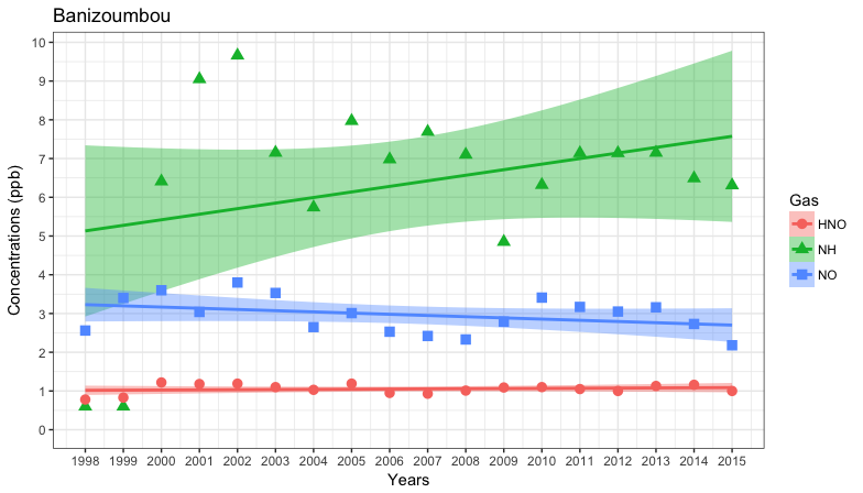
I want to add 3 linear regression lines to 3 different groups of points in the same graph. I initially plotted these 3 distincts scatter plot with geom_point(), but I don't know how to do that.
Here is an example of my data:
Years ppb Gas
1998 2,56 NO
1999 3,40 NO
2000 3,60 NO
2001 3,04 NO
2002 3,80 NO
2003 3,53 NO
2004 2,65 NO
2005 3,01 NO
2006 2,53 NO
2007 2,42 NO
2008 2,33 NO
2009 2,79 NO
2010 3,41 NO
2011 3,17 NO
2012 3,05 NO
2013 3,16 NO
2014 2,73 NO
2015 2,18 NO
1998 0,60 NH
1999 0,60 NH
2000 6,41 NH
2001 9,05 NH
2002 9,66 NH
2003 7,15 NH
2004 5,74 NH
2005 7,97 NH
2006 6,98 NH
2007 7,69 NH
2008 7,10 NH
2009 4,85 NH
2010 6,32 NH
2011 7,14 NH
2012 7,14 NH
2013 7,15 NH
2014 6,49 NH
2015 6,31 NH
1998 0,78 HNO
1999 0,83 HNO
2000 1,22 HNO
2001 1,18 HNO
2002 1,19 HNO
2003 1,10 HNO
2004 1,03 HNO
2005 1,19 HNO
2006 0,95 HNO
2007 0,93 HNO
2008 1,01 HNO
2009 1,09 HNO
2010 1,10 HNO
2011 1,05 HNO
2012 1,00 HNO
2013 1,13 HNO
2014 1,16 HNO
2015 1,00 HNO

Here's my code :

library(ggplot2)
xyears <- test$Years
y <- test$ppb
group <- test$Gas
p <- ggplot(test) +
aes(Years, ppb, shape = Gas) +
geom_point(aes(colour = Gas), size = 3) +
geom_point(colour = "grey90", size = 1.5) +
theme_bw() + 
xlab("Years") +
ylab("Concentrations (ppb)") +
ggtitle("Banizoumbou") + 
scale_y_continuous(breaks = seq(0 , 10, 1)) + 
scale_x_continuous(breaks = seq(1998, 2015, 1)) 

Thanks !

You can add the regression lines with geom_smooth:

ggplot(test, aes(Years, ppb, shape=Gas, colour=Gas, fill=Gas)) +
  geom_smooth(method="lm") +
  geom_point(size=3) +
  theme_bw() + 
  xlab("Years") +
  ylab("Concentrations (ppb)") +
  ggtitle("Banizoumbou") + 
  expand_limits(y=0) +
  scale_y_continuous(breaks = 0:10) + 
  scale_x_continuous(breaks = 1998:2015)

3 Likes

Is there a solution to write for example NO2, NH3 and HNO3 with 2 and 3 in subscript in the legend?

Thanks !

Yup! You can do so with R's plotmath system for mathematical annotation.

Note that you need to provide the same labels to all three of the aesthetics that you've mapped to Gas.

labels_Gas <- c(
  "HNO" = expression(HNO[3]), 
  "NH" = expression(NH[3]), 
  "NO" = expression(NO[2])
)

ggplot(test, aes(Years, ppb, shape=Gas, colour=Gas, fill=Gas)) +
  geom_smooth(method="lm") +
  geom_point(size=3) +
  theme_bw() + 
  xlab("Years") +
  ylab("Concentrations (ppb)") +
  ggtitle("Banizoumbou") + 
  expand_limits(y=0) +
  scale_y_continuous(breaks = 0:10) + 
  scale_x_continuous(breaks = 1998:2015) + 
  scale_shape(labels = labels_Gas) + 
  scale_colour_discrete(labels = labels_Gas) + 
  scale_fill_discrete(labels = labels_Gas)

reprex-body-1

You could also choose to simplify the legend by having some aesthetics left out:

ggplot(test, aes(Years, ppb, shape=Gas, colour=Gas, fill=Gas)) +
  geom_smooth(method="lm", show.legend = FALSE) +
  geom_point(size=3) +
  theme_bw() + 
  xlab("Years") +
  ylab("Concentrations (ppb)") +
  ggtitle("Banizoumbou") + 
  expand_limits(y=0) +
  scale_y_continuous(breaks = 0:10) + 
  scale_x_continuous(breaks = 1998:2015) + 
  scale_shape(labels = labels_Gas) + 
  scale_colour_discrete(labels = labels_Gas) + 
  guides(fill = "none")

9328_2

4 Likes