Hi, I am using the 'gbm' package to get average propensity scores. The code works fine. But the problem is that mean of the control group doesn't change after including the weights. I know that this may be the problem with the dataset I am using. But, I want to be sure that I didn't do any mistakes in the code.
I have added the code. Here, y is the outcome/response variable and z is the treatment variable and x is the data frame containing all other covariates. I uploaded a screenshot of the results.
# load the gbm library into memory
library(gbm)
library(knitr)
library(haven)
# the following code identifies the response variable
i.y <- which(names(mydata)=="y")
# call gbm
gbm1 <- gbm(z~., # predicts z from all other variables
data=mydata[,-i.y], # the dataset dropping y
distribution="bernoulli", # indicates logistic regression
n.trees=20000, # runs for 20,000 iterations
shrinkage=0.0005, # sets the shrinkage parameter
interaction.depth=4, # maximum allowed interaction degree
bag.fraction=0.5, # sets fraction used for Friedman's
# random subsampling of the data
train.fraction=1.0, # train.fraction<1.0 allows for
# out-of-sample prediction for
# stopping the algorithm
n.minobsinnode=10) # minimum node size for trees
# The following two functions are useful for choosing the GBM function
# that minimizes ASAM
# std.diff is a helper function that computes the standardized
# absolute mean difference which is used in ASAM
# u is the variable to be tested, a covariate to be balanced by
# propensity score weighting
# z is a vector of 0s and 1s indicating treatment assignment
# w is a vector of the propensity score weights
std.diff <- function(u,z,w)
{
# for variables other than unordered categorical variables
# compute mean differences
# mean() is a function to calculate means
# u[z==1] selected values of u where z=1
# mean(u[z==1]) gives the mean of u for the treatment group
# weighted.mean() is a function to calculate weighted mean
# the option--na.rm controls missing values
# u[z==0],w[z==0] select values of u and the weights for the comparison
# group
# weighted.mean(u[z==0],w[z==0],na.rm=TRUE) gives the weighted mean for
# the comparison group
# abs() is a function to calculate absolute values
# sd() is a function to caluculate standard deviations from a sample
# sd(u[z==1], na.rm=T) calculates the standard deviation for the
# treatment group
if(!is.factor(u))
{
sd1 <- sd(u[z==1], na.rm=T)
if(sd1 > 0)
{
result <- abs(mean(u[z==1],na.rm=TRUE)-
weighted.mean(u[z==0],w[z==0],na.rm=TRUE))/sd1
} else
{
result <- 0
warning("Covariate with standard deviation 0.")
}
}
# for factors compute differences in percentages in each category
# for(u.level in levels(u) creates a loop that repeats for each level of
# the categorical variable
# as.numeric(u==u.level) creates as 0-1 variable indicating u is equal to
# u.level the current level of the for loop
# std.diff(as.numeric(u==u.level),z,w)) calculates the absolute
# standardized difference of the indicator variable
else
{
result <- NULL
for(u.level in levels(u))
{
result <- c(result, std.diff(as.numeric(u==u.level),z,w))
}
}
return(result)
}
# asam function computes the ASAM for the gbm model after "i" iterations
# gbm1 is the gbm model for the propensity score
# x is a data frame with only the covariates
# z is a vector of 0s and 1s indicating treatment assignment
asam <- function(i,gbm1,x,z)
{
cat(i,"\n") # prints the iteration number
i <- floor(i) # makes sure that i is an integer
# predict(gbm1, x, i) provides predicted values on the log-odds of
# treatment for the gbm model with i iterations at the values of x
# exp(predict(gbm1, x, i)) calculates the odds treatment or the weight
# from the predicted values
w <- exp(predict(gbm1, x, i))
# assign treatment cases a weight of 1
w[z==1] <- 1
# sapply repeats calculation of std.diff for each variable (column) of x
# unlist is an R function for managing data structures
# mean(unlist(sapply(x, std.diff, z=z, w=w))) calculates the mean of the
# standardized differences for all variables in x or ASAM
return(mean(unlist(sapply(x, std.diff, z=z, w=w))))
}
# find the number of iterations that minimizes asam
# create indicator j.drop for the response, treatment indicator and weight
# variable, these variables are exclude from the covariates
40
j.drop <- match(c("y","z","w"),names(mydata))
j.drop <- j.drop[!is.na(j.drop)]
# optimize is an R function for maximizing a function
# we use optimize to find the number of iterations of the gbm
# algorithm that maximizes asam
# interval and tol are parameters of the optimize function
# gbm, x and z are parameters of that optimizes passes to the
# asam function as fixed values so asam is a function only of i
# and optimize maximizes asam as function of i as desired
opt <- optimize(asam, # optimize asam
interval=c(100, 20000), # range in which to search
tol=1, # get within one iteration
gbm1=gbm1, # the propensity score model
x=mydata[,-j.drop], # data dropping y, z, w (if there)
z=mydata$z) # the treatment assignment indicator
# store the best number of iterations
best.asam.iter <- opt$minimum
# estimate the training R2
r2 <- with(gbm1, 1 - train.error[best.asam.iter]/
mean(mydata$z*initF - log(1+exp(initF))))
# estimate Average Treatment Effect on the Treated
# create a weight w using the optimal gbm model
# exp( predict(gbm1, mydata[mydata$z==0,], best.asam.iter) )
# calculates
# the weights (the odds of treatment assignment) based on optimal gbm model
# for the comparison cases
mydata$w <- rep(1,nrow(mydata))
mydata$w[mydata$z==0] <-
exp( predict(gbm1, mydata[mydata$z==0,], best.asam.iter) )
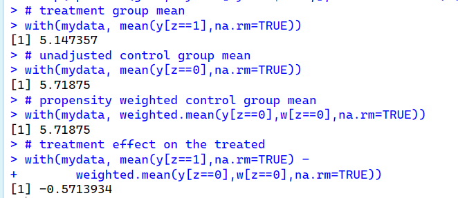
# treatment group mean
with(mydata, mean(y[z==1],na.rm=TRUE))
# unadjusted control group mean
with(mydata, mean(y[z==0],na.rm=TRUE))
# propensity weighted control group mean
with(mydata, weighted.mean(y[z==0],w[z==0],na.rm=TRUE))
# treatment effect on the treated
with(mydata, mean(y[z==1],na.rm=TRUE) -
weighted.mean(y[z==0],w[z==0],na.rm=TRUE))