Scatterplot of one x and 5 y / adjustment of example code

Hello everybody,

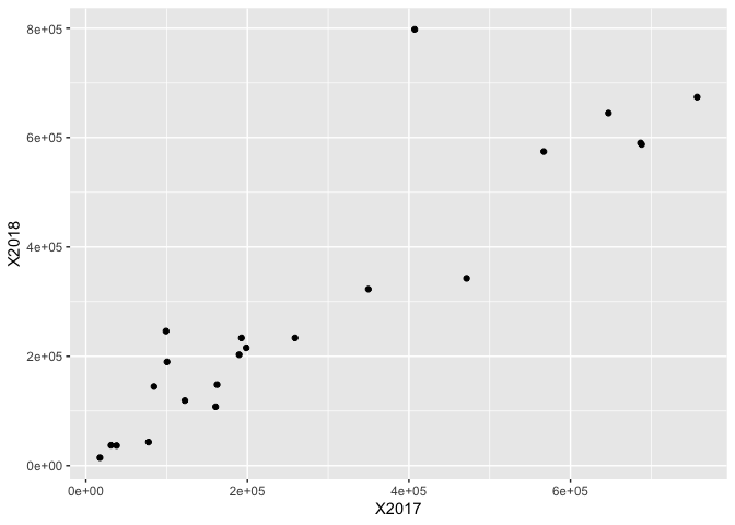
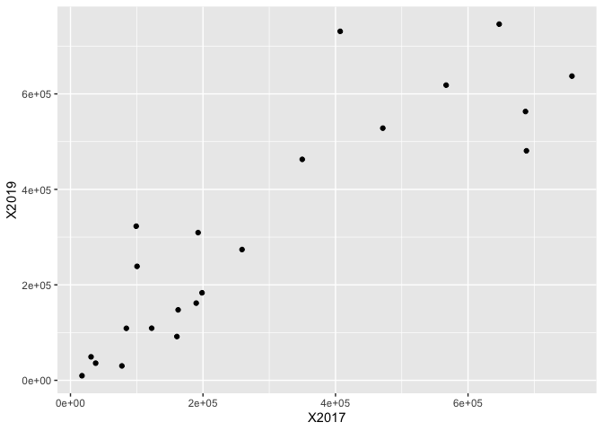
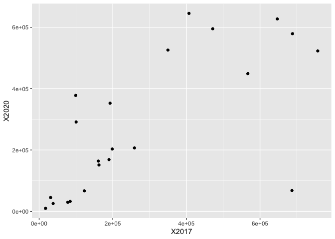
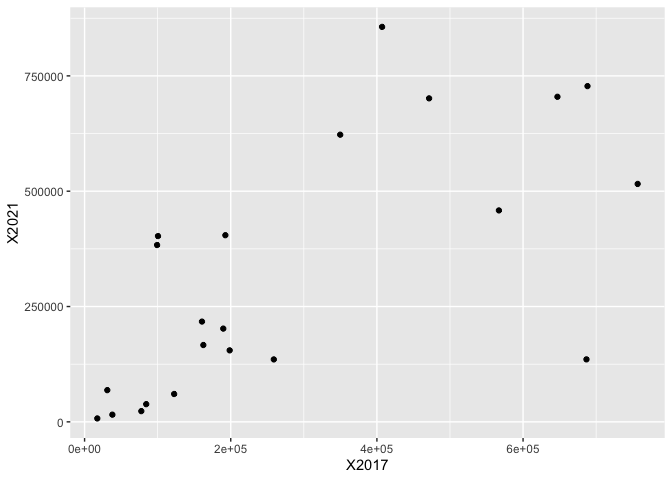
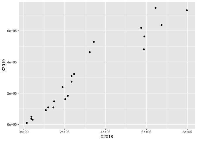
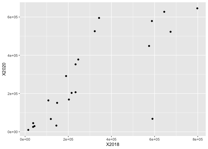
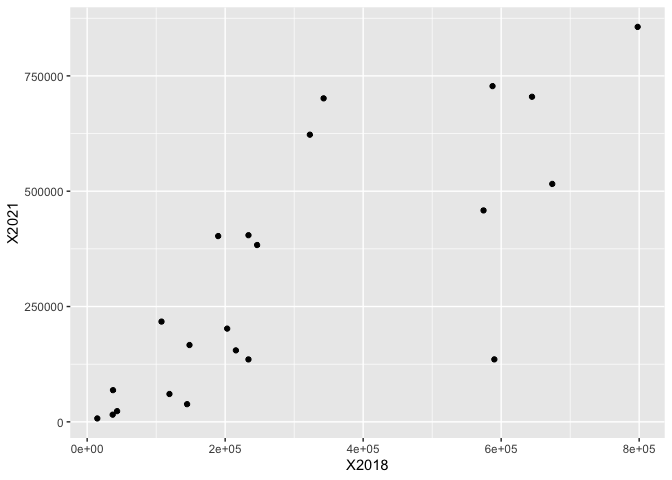
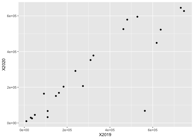
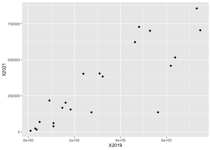
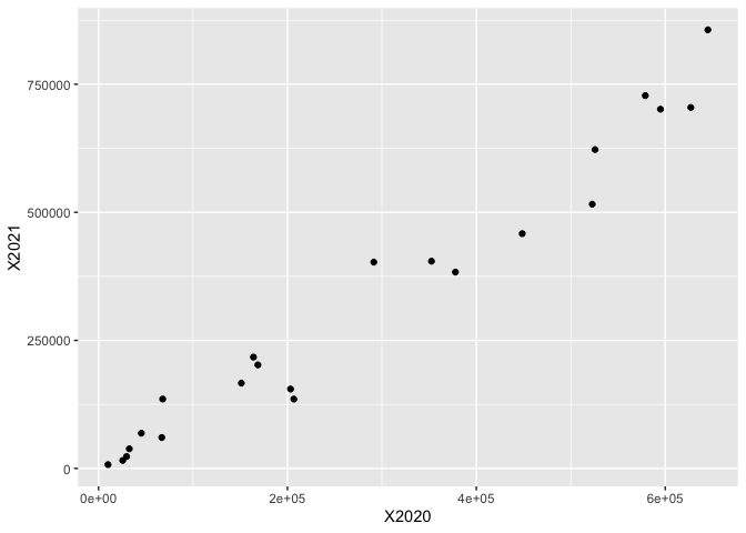
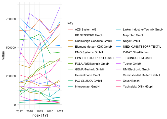
as a final challenge, I want to create a scatterplot of the dataset below, with Companies as x and the corresponding values as y. I found the ideal example code of the iris dataset based on dplyr and tidyr:

exampleData <-
iris %>%
filter(Species == "setosa") %>%
slice(1:10) %>%
select(Sepal.Length:Petal.Length)

exampleData

toPlot <-
exampleData %>%
gather(sepalMeasure, size, -Petal.Length)

toPlot %>%
ggplot(aes(x = Petal.Length
, y = size
, col = sepalMeasure)) +
geom_point()

I´m desperately trying to adjust the code, but I just don´t get it fixed without any help.
Thank you already for any advice and support!!

data.frame(
stringsAsFactors = FALSE,
Company = c("NIED KUNSTSTOFF-TEXTIL",
"Nagel GmbH","BD SENSORS GmbH","TECHNOCHEM GMBH",
"Xaver Bosch","GEMA-Technik GmbH","Linker Industrie-Technik GmbH",
"Element Metech KDK GmbH","Heinzelmann GmbH",
"Intercontact GmbH","IAG GLUSKA GmbH ","AZS System AG",
"UM Electronic GmbH","Maprotec GmbH",
"CubiDesign Gehäuse GmbH","Q-BAT Oberflächen","Tucker GmbH","EMO Systems GmbH",
"EPN ELECTROPRINT GmbH","FOLA Abfülltechnik GmbH",
"YachtelektrONik Höppli","Vereinsbedarf Deitert GmbH"),
X2017 = c(756823,688146,647021,407077,
471399,566944,686736,349779,84330,122540,17397,
38019,77618,31067,189772,198546,162485,160636,192630,
99207,258933,100464),
X2018 = c(674026,587493,644712,797846,
342685,574444,590111,322751,144808,119248,14684,
36982,43380,37444,202914,215543,148313,107733,
233774,246281,233752,189849),
X2019 = c(637241,480784,746121,731033,
528222,618359,563104,462867,108934,109194,9647,
35960,30213,49179,161728,183365,147625,91725,309424,
322866,273941,238745),
X2020 = c(522727,578899,627080,645161,
594989,448580,67919,525696,32547,66967,9998,25591,
29635,45296,168686,203288,151228,164011,352489,
377846,206766,291408),
X2021 = c(515765,727793,704699,856202,
701297,458338,135450,622501,38381,60398,7414,
15591,23253,68760,202138,154995,166553,217375,404617,
383349,135356,402740)
)

The sample is a scatterplot of two continuous variables of a subset of one of three species with multiple observations; the bank data has four continuous variables of 22 companies with single observations of each continuous variable. These are incommensurate.

To just do a scatterplot, pick any pair of the X2... variables. If these represent years, a scatterplot will not be as informative as a time series plot.

library(dplyr)
#> 
#> Attaching package: 'dplyr'
#> The following objects are masked from 'package:stats':
#> 
#>     filter, lag
#> The following objects are masked from 'package:base':
#> 
#>     intersect, setdiff, setequal, union
library(ggplot2)

d <- data.frame(
  stringsAsFactors = FALSE,
  Company = c("NIED KUNSTSTOFF-TEXTIL",
              "Nagel GmbH","BD SENSORS GmbH","TECHNOCHEM GMBH",
              "Xaver Bosch","GEMA-Technik GmbH","Linker Industrie-Technik GmbH",
              "Element Metech KDK GmbH","Heinzelmann GmbH",
              "Intercontact GmbH","IAG GLUSKA GmbH ","AZS System AG",
              "UM Electronic GmbH","Maprotec GmbH",
              "CubiDesign Gehäuse GmbH","Q-BAT Oberflächen","Tucker GmbH","EMO Systems GmbH",
              "EPN ELECTROPRINT GmbH","FOLA Abfülltechnik GmbH",
              "YachtelektrONik Höppli","Vereinsbedarf Deitert GmbH"),
  X2017 = c(756823,688146,647021,407077,
            471399,566944,686736,349779,84330,122540,17397,
            38019,77618,31067,189772,198546,162485,160636,192630,
            99207,258933,100464),
  X2018 = c(674026,587493,644712,797846,
            342685,574444,590111,322751,144808,119248,14684,
            36982,43380,37444,202914,215543,148313,107733,
            233774,246281,233752,189849),
  X2019 = c(637241,480784,746121,731033,
            528222,618359,563104,462867,108934,109194,9647,
            35960,30213,49179,161728,183365,147625,91725,309424,
            322866,273941,238745),
  X2020 = c(522727,578899,627080,645161,
            594989,448580,67919,525696,32547,66967,9998,25591,
            29635,45296,168686,203288,151228,164011,352489,
            377846,206766,291408),
  X2021 = c(515765,727793,704699,856202,
            701297,458338,135450,622501,38381,60398,7414,
            15591,23253,68760,202138,154995,166553,217375,404617,
            383349,135356,402740)
)

ggplot(d,aes(X2017,X2018)) + geom_point()

ggplot(d,aes(X2017,X2019)) + geom_point()

ggplot(d,aes(X2017,X2020)) + geom_point()

ggplot(d,aes(X2017,X2021)) + geom_point()

ggplot(d,aes(X2018,X2019)) + geom_point()

ggplot(d,aes(X2018,X2020)) + geom_point()

ggplot(d,aes(X2018,X2021)) + geom_point()

ggplot(d,aes(X2019,X2020)) + geom_point()

ggplot(d,aes(X2019,X2021)) + geom_point()

ggplot(d,aes(X2020,X2021)) + geom_point()

Created on 2023-03-26 with reprex v2.0.2

Hello @technocrat,

thank you very much (again) for your time, help and explanation. Indeed, the X2.. variables represent years. Despite the drawbacks (and for reasons of space), the data sadly have to be united in a single graph.

Here is a single-graph display. It presents some challenges in distinguishing among the large number of series.

library(fpp3)
#> ── Attaching packages ────────────────────────────────────────────── fpp3 0.5 ──
#> ✔ tibble      3.2.1     ✔ tsibble     1.1.3
#> ✔ dplyr       1.1.1     ✔ tsibbledata 0.4.1
#> ✔ tidyr       1.3.0     ✔ feasts      0.3.1
#> ✔ lubridate   1.9.2     ✔ fable       0.3.3
#> ✔ ggplot2     3.4.1     ✔ fabletools  0.3.2
#> ── Conflicts ───────────────────────────────────────────────── fpp3_conflicts ──
#> ✖ lubridate::date()    masks base::date()
#> ✖ dplyr::filter()      masks stats::filter()
#> ✖ tsibble::intersect() masks base::intersect()
#> ✖ tsibble::interval()  masks lubridate::interval()
#> ✖ dplyr::lag()         masks stats::lag()
#> ✖ tsibble::setdiff()   masks base::setdiff()
#> ✖ tsibble::union()     masks base::union()
d <- data.frame(
  Company = c("NIED KUNSTSTOFF-TEXTIL",
              "Nagel GmbH","BD SENSORS GmbH","TECHNOCHEM GMBH",
              "Xaver Bosch","GEMA-Technik GmbH","Linker Industrie-Technik GmbH",
              "Element Metech KDK GmbH","Heinzelmann GmbH",
              "Intercontact GmbH","IAG GLUSKA GmbH ","AZS System AG",
              "UM Electronic GmbH","Maprotec GmbH",
              "CubiDesign Gehäuse GmbH","Q-BAT Oberflächen","Tucker GmbH","EMO Systems GmbH",
              "EPN ELECTROPRINT GmbH","FOLA Abfülltechnik GmbH",
              "YachtelektrONik Höppli","Vereinsbedarf Deitert GmbH"),
  X2017 = c(756823,688146,647021,407077,
            471399,566944,686736,349779,84330,122540,17397,
            38019,77618,31067,189772,198546,162485,160636,192630,
            99207,258933,100464),
  X2018 = c(674026,587493,644712,797846,
            342685,574444,590111,322751,144808,119248,14684,
            36982,43380,37444,202914,215543,148313,107733,
            233774,246281,233752,189849),
  X2019 = c(637241,480784,746121,731033,
            528222,618359,563104,462867,108934,109194,9647,
            35960,30213,49179,161728,183365,147625,91725,309424,
            322866,273941,238745),
  X2020 = c(522727,578899,627080,645161,
            594989,448580,67919,525696,32547,66967,9998,25591,
            29635,45296,168686,203288,151228,164011,352489,
            377846,206766,291408),
  X2021 = c(515765,727793,704699,856202,
            701297,458338,135450,622501,38381,60398,7414,
            15591,23253,68760,202138,154995,166553,217375,404617,
            383349,135356,402740)
)

# transpose and convert back to data frame
d_ts <- as.data.frame(t(d))
# convert from character to numeric 
d_ts <- sapply(d_ts,as.numeric)
#> Warning in lapply(X = X, FUN = FUN, ...): NAs introduced by coercion

#> Warning in lapply(X = X, FUN = FUN, ...): NAs introduced by coercion

#> Warning in lapply(X = X, FUN = FUN, ...): NAs introduced by coercion

#> Warning in lapply(X = X, FUN = FUN, ...): NAs introduced by coercion

#> Warning in lapply(X = X, FUN = FUN, ...): NAs introduced by coercion

#> Warning in lapply(X = X, FUN = FUN, ...): NAs introduced by coercion

#> Warning in lapply(X = X, FUN = FUN, ...): NAs introduced by coercion

#> Warning in lapply(X = X, FUN = FUN, ...): NAs introduced by coercion

#> Warning in lapply(X = X, FUN = FUN, ...): NAs introduced by coercion

#> Warning in lapply(X = X, FUN = FUN, ...): NAs introduced by coercion

#> Warning in lapply(X = X, FUN = FUN, ...): NAs introduced by coercion

#> Warning in lapply(X = X, FUN = FUN, ...): NAs introduced by coercion

#> Warning in lapply(X = X, FUN = FUN, ...): NAs introduced by coercion

#> Warning in lapply(X = X, FUN = FUN, ...): NAs introduced by coercion

#> Warning in lapply(X = X, FUN = FUN, ...): NAs introduced by coercion

#> Warning in lapply(X = X, FUN = FUN, ...): NAs introduced by coercion

#> Warning in lapply(X = X, FUN = FUN, ...): NAs introduced by coercion

#> Warning in lapply(X = X, FUN = FUN, ...): NAs introduced by coercion

#> Warning in lapply(X = X, FUN = FUN, ...): NAs introduced by coercion

#> Warning in lapply(X = X, FUN = FUN, ...): NAs introduced by coercion

#> Warning in lapply(X = X, FUN = FUN, ...): NAs introduced by coercion

#> Warning in lapply(X = X, FUN = FUN, ...): NAs introduced by coercion
# remove NA to row
d_ts <- d_ts[-1,]
# restore Company names
colnames(d_ts) <- d$Company
# create time series object
d_ts <- ts(d_ts,start = 2017, frequency = 1)
# convert to tidyverse version
d_tsb <- as_tsibble(d_ts)
# plot all Companies
autoplot(d_tsb) + theme_minimal()
#> Plot variable not specified, automatically selected `.vars = value`

Created on 2023-03-27 with reprex v2.0.2

I can´t thank you enough @technocrat! You saved a qualitative researcher´s life!

1 Like

Still, consider subsets into batches of 7,7 and 8 to improve legibility if you can escape the single plot constraint

This topic was automatically closed 42 days after the last reply. New replies are no longer allowed.

If you have a query related to it or one of the replies, start a new topic and refer back with a link.