I can revisit this later. I may be able to figure it out. I wanted to try to set up the initial_split function. It still keeps returning an error message
OK.
The last I saw of your initial_split() code, you were using strata = y.
split <- initial_split(dataset2, prop = 0.8, strata = y)
Since there is not column named y, the code throws an error. Making a variable named y doesn't make sense to me. If you want to use the strata argument, it should get the name of a column in your data set.
But that's what I attempted to do. I assigned y the name of the column 'user_type' and it still didn't work.
Here are the two different codes I ran:
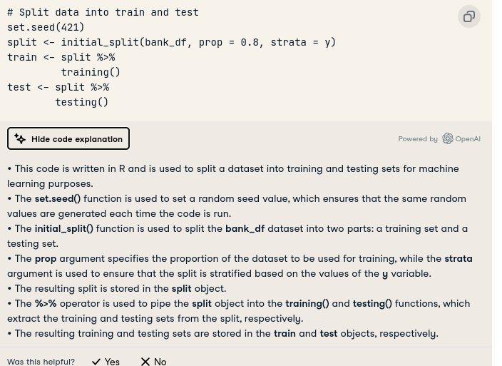
Split data into train and test
set.seed(421)
split <- initial_split(dataset2, prop = 0.8, strata = dataset2$user_type)
Error inmc_cv():
! Selections can't have missing values.
Runrlang::last_trace()to see where the error occurred.Split data into train and test
set.seed(421)
split <- initial_split(dataset2, prop = 0.8, strata = user_type)
Warning message:
Too little data to stratify.
• Resampling will be unstratified.
train <-split %>%
- training()
test <- split %>%
- testing()
Heres the tutorial I tried to follow
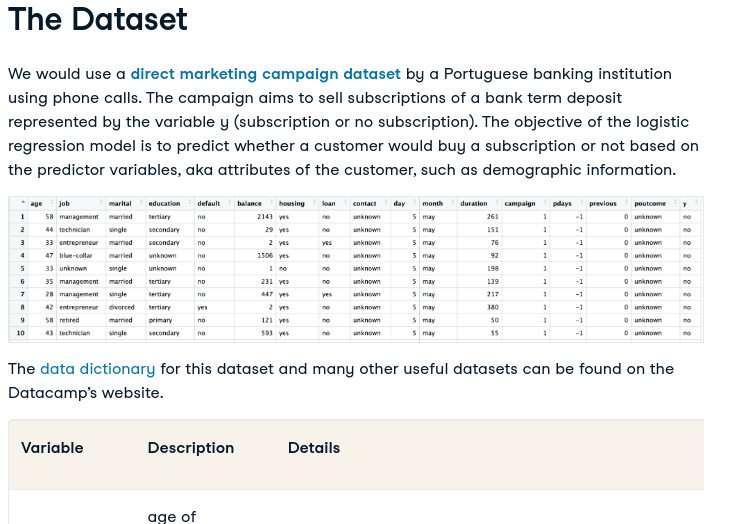
The dataset is defined here in this article https://www.datacamp.com/tutorial/logistic-regression-R
It's somewhat similar, in that they are trying to determine subscriptions as well.
Your second attempt ran with no errors. You do get a warning. The code ran and you should have the train and test data sets. Do those meet your needs?
set.seed(421)
split <- initial_split(dataset2, prop = 0.8, strata = user_type)
#Warning message:
#  Too little data to stratify.
#• Resampling will be unstratified.
train <-split %>%

  training()

test <- split %>%

  testing()
I have not used tidymodels and I'm not familiar with the functions in rsample. My guess is that by setting strata = user_type, the function first runs user_type through the function make_strata(). Here is some documentation for that function.
Read that carefully, particularly looking at the examples. It makes sense that user_type can't be stratified.
As for the example you have been following, without knowing where that comes from and examining the details, I can't comment on why that code works with that data. And, as I said, I don't use these functions, so my comments are unlikely to be very valuable. It makes sense that different data sets need different argument choices.
Thank you I will review this. I don't know why this keep happening but I tried to follow up my last post with a link to an article I was referencing.
They keep temporarily hiding it to review it for spam.
Here it is:
Thank you I will review this one moment. Also, I keep trying to follow-up my post with a link to the article on Data Camp I was referencing, It is called Logistic Regression in R Tutorial.
Each time I post this link I received a notification from Community stating "Akismet has temporarily hidden your post' I guess because because it believes it to be spam?
One moment I can screenshot some of it here,


Hmm, the variable y is also binary like your user_type. I don't know why initial_split is throwing a warning about "too little data". You have a lot of data in each category, judging from your plots,
1 Like
I guess my question here is how is that the dataset is considered too small if there is 365069 rows of observations? And the y variable is similar to this dataset's in that it is determining whether a customer has purchased a subscription (yes) or not.
The code did not meet my needs because I thought it was supposed to return a value?
I proceeded in the steps and next ran the following code:
install.packages("glmnet")
install.packages("classification")
library(glmnet)
library(classification)
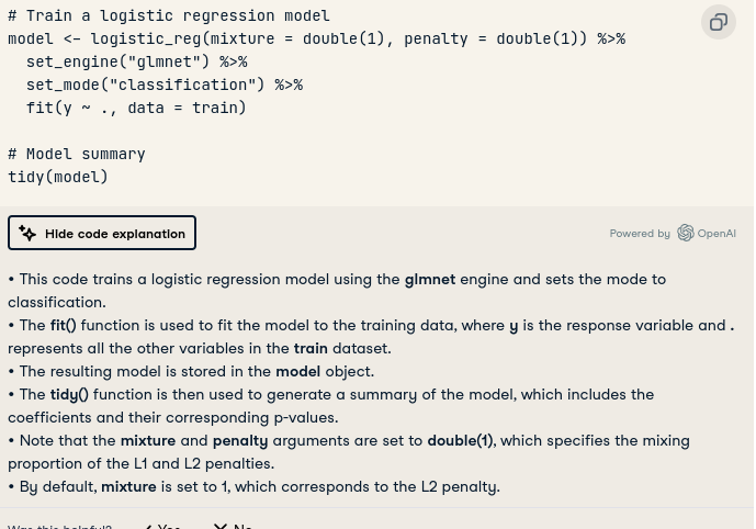
Train a logistic regression model
model <- logistic_reg(mixture = double(1), penalty = double(1)) %>%
set_engine("glmnet") %>%
set_mode("classification") %>%
fit(dataset2$user_type ~ ., data = train)
Error Message Returned:
Warning in install.packages :
package ‘classification’ is not available for this version of R
A version of this package for your version of R might be available elsewhere,
see the ideas at
library(glmnet)
Loading required package: Matrix
Attaching package: ‘Matrix’
The following objects are masked from ‘package:tidyr’:
expand, pack, unpack
Loaded glmnet 4.1-8
library(classification)
Error in library(classification) :
there is no package called ‘classification’Train a logistic regression model
model <- logistic_reg(mixture = double(1), penalty = double(1)) %>%
- set_engine("glmnet") %>%
- set_mode("classification") %>%
- fit(dataset2$user_type ~ ., data = train)
Error in model.frame.default(formula, data) :
variable lengths differ (found for 'trip_id')
** trip_id's are meant to be different. is there a way around this to run the "train a logistic model" ?
I attemped to change the y variable from dataset2$user_type to user_type to see if that would make a difference.
Train a logistic regression model
model <- logistic_reg(mixture = double(1), penalty = double(1)) %>%
- set_engine("glmnet") %>%
- set_mode("classification") %>%
- fit(user_type ~ ., data = train)
Returned Error Message: Error in contrasts<-(*tmp*, value = contr.funs[1 + isOF[nn]]) :
contrasts can be applied only to factors with 2 or more levels

@FJCC So I figured maybe the NA values for user_type and ride_length impacted the initial splitting so I reran the the code from the beginning and then the assigned the factor.
It did not work.
Would you know where to go from here ?
I've lost track of all the steps in your process. Please show all of your code from the step where you read in the data to the point where you first see that user_type and ride_length are filled with NA. Place that code between lines with three back ticks.
```
Code goes here
```
The back tick key is immediately to the left of the 1 key on a standard US keyboard. It is different than an apostrophe. Back tick = `, apostrophe = '.
Separately, show the first few rows of the data set immediately after you read it in. If that data frame is named dataset2, run
dput(head(dataset2, 10))
Post the output of that between lines with three back ticks.
@FJCC Sure, no problem,
Here is the code that was ran in the console.
 install.packages("tidyverse")
Installing package into ‘/cloud/lib/x86_64-pc-linux-gnu-library/4.3’
(as ‘lib’ is unspecified)
trying URL 'http://rspm/default/__linux__/focal/latest/src/contrib/tidyverse_2.0.0.tar.gz'
Content type 'application/x-gzip' length 425237 bytes (415 KB)
==================================================
downloaded 415 KB

* installing *binary* package ‘tidyverse’ ...
* DONE (tidyverse)

The downloaded source packages are in
	‘/tmp/RtmpCbCIX9/downloaded_packages’
> install.packages("tidymodels")
Error in install.packages : Updating loaded packages
> library(tidymodels)
> install.packages("tidymodels")
Installing package into ‘/cloud/lib/x86_64-pc-linux-gnu-library/4.3’
(as ‘lib’ is unspecified)
trying URL 'http://rspm/default/__linux__/focal/latest/src/contrib/tidymodels_1.1.1.tar.gz'
Content type 'application/x-gzip' length 86487 bytes (84 KB)
==================================================
downloaded 84 KB

* installing *binary* package ‘tidymodels’ ...
* DONE (tidymodels)

The downloaded source packages are in
	‘/tmp/RtmpCbCIX9/downloaded_packages’
> #Read the dataset and convert the variable to a factor
> dataset2 <- read.csv("Bike_Trips_2019.csv")
> dataset2$user_type =as.factor(dataset2$user_type)
> View(dataset2)
> install.packages("ggplot2")
Error in install.packages : Updating loaded packages
> library(ggplot2)
> install.packages("ggplot2")
Installing package into ‘/cloud/lib/x86_64-pc-linux-gnu-library/4.3’
(as ‘lib’ is unspecified)
trying URL 'http://rspm/default/__linux__/focal/latest/src/contrib/ggplot2_3.5.0.tar.gz'
Content type 'application/x-gzip' length 4809806 bytes (4.6 MB)
==================================================
downloaded 4.6 MB

* installing *binary* package ‘ggplot2’ ...
* DONE (ggplot2)

The downloaded source packages are in
	‘/tmp/RtmpCbCIX9/downloaded_packages’
> dataset2$user_type <- factor(dataset2$user_type, levels = c("Customer", "Subscriber"), labels = c("no","yes"))
> ggplot(dataset2,aes(birthyear, fill = user_type)) +
+   geom_bar()+
+   coord_flip()
Warning message:
Removed 18023 rows containing non-finite outside the scale range
(`stat_count()`).
> install.packages("rsample")
Error in install.packages : Updating loaded packages
> library(rsample)
> install.packages("rsample")
Installing package into ‘/cloud/lib/x86_64-pc-linux-gnu-library/4.3’
(as ‘lib’ is unspecified)
trying URL 'http://rspm/default/__linux__/focal/latest/src/contrib/rsample_1.2.0.tar.gz'
Content type 'application/x-gzip' length 522443 bytes (510 KB)
==================================================
downloaded 510 KB

* installing *binary* package ‘rsample’ ...
* DONE (rsample)

The downloaded source packages are in
	‘/tmp/RtmpCbCIX9/downloaded_packages’
> y <- dataset2$user_type
> > # Split data into train and test
> set.seed(421)
> split <- initial_split(dataset2, prop = 0.8, strata = y)
Error in `mc_cv()`:
! Can't subset columns that don't exist.
✖ Columns `yes`, `yes`, `yes`, `yes`, `yes`, etc. don't exist.
Run `rlang::last_trace()` to see where the error occurred.
Warning message:
Using an external vector in selections was deprecated in tidyselect 1.1.0.
ℹ Please use `all_of()` or `any_of()` instead.
  # Was:
  data %>% select(y)

  # Now:
  data %>% select(all_of(y))

See <https://tidyselect.r-lib.org/reference/faq-external-vector.html>.
This warning is displayed once every 8 hours.
Call `lifecycle::last_lifecycle_warnings()` to see where this warning was generated.
> dataset2$ride_length <- factor(dataset2$ride_length, levels = c("Customer", "Subscriber"),labels = c("no", "yes"))
> ggplot(dataset2,aes(gender, fill = user_type))+
+   geom_bar()+
+   coord_flip()+
+ dataset2$ride_length <- factor(dataset2$ride_length, levels = c("Customer", "Subscriber"),labels = c("no", "yes"))
Error in ggplot(dataset2, aes(gender, fill = user_type)) + geom_bar() +  :
  could not find function "+<-"
> dataset2$ride_length <- factor(dataset2$ride_length, levels = c("Customer", "Subscriber"),labels = c("no", "yes"))
> ggplot(dataset2,aes(gender, fill = ride_length))+
+   geom_bar()+
+   coord_flip()
Error in `palette()`:
! Must request at least one colour from a hue
  palette.
Run `rlang::last_trace()` to see where the error occurred.
> dataset2$user_type <- factor(dataset2$user_type, levels = c("Customer", "Subscriber"), labels = c("no","yes"))
> ggplot(dataset2,aes(day_of_week, fill = ride_length)) +
+   geom_bar()+
+   coord_flip()
Error in `palette()`:
! Must request at least one colour from a hue
  palette.
Run `rlang::last_trace()` to see where the error occurred.
> dataset2$user_type <- factor(dataset2$user_type, levels = c("Customer", "Subscriber"), labels = c("no","yes"))
> ggplot(dataset2,aes(ride_length, fill = user_type)) +
+   geom_bar()+
+   coord_flip()
Error in `palette()`:
! Must request at least one colour from a hue
  palette.
Run `rlang::last_trace()` to see where the error occurred.
> # Split data into train and test
> set.seed(421)
> split <- initial_split(dataset2, prop = 0.8, strata = dataset2$user_type)
Error in `mc_cv()`:
! Selections can't have missing values.
Run `rlang::last_trace()` to see where the error occurred.
> # Split data into train and test
> set.seed(421)
> split <- initial_split(dataset2, prop = 0.8, strata = user_type)
Warning message:
Too little data to stratify.
• Resampling will be unstratified.
> train <-split %>%
+   training()
> test <- split %>%
+   testing()
> # Split data into train and test
> set.seed(365069)
> split <- initial_split(dataset2, prop = 0.8, strata = user_type)
Warning message:
Too little data to stratify.
• Resampling will be unstratified.
> train <-split %>%
+   training()
> test <- split %>%
+   testing()
> # Split data into train and test
> set.seed(421)
> split <- initial_split(dataset2, prop = 0.8, strata = ride_length)
Warning message:
Too little data to stratify.
• Resampling will be unstratified.
> train <-split %>%
+   training()
> test <- split %>%
+   testing()
> # Split data into train and test
> set.seed(421)
> split <- initial_split(dataset2, prop = 1, strata = ride_length)
Error in `mc_splits()`:
! `prop` must be a number on (0, 1).
Run `rlang::last_trace()` to see where the error occurred.
> # Split data into train and test
> set.seed(421)
> split <- initial_split(dataset2, prop =.9, strata = ride_length)
Warning message:
Too little data to stratify.
• Resampling will be unstratified.
> train <-split %>%
+   training()
> test <- split %>%
+   testing()
> # Split data into train and test
> set.seed(421)
> split <- initial_split(dataset2, prop =.5, strata = ride_length)
Warning message:
Too little data to stratify.
• Resampling will be unstratified.
> train <-split %>%
+   training()
> test <- split %>%
+   testing()
> # Train a logistic regression model
> model <- logistic_reg(mixture = double(1), penalty = double(1)) %>%
+   set_engine("glmnet") %>%
+   set_mode("classification") %>%
+   fit(user_type ~ ., dataset2 = train)
Error in fit.model_spec(., user_type ~ ., dataset2 = train) :
  argument "data" is missing, with no default
> # Train a logistic regression model
> model <- logistic_reg(mixture = double(1), penalty = double(1)) %>%
+   set_engine("glmnet") %>%
+   set_mode("classification") %>%
+   fit(dataset2$user_type ~ ., dataset2 = train)
Error in fit.model_spec(., dataset2$user_type ~ ., dataset2 = train) :
  argument "data" is missing, with no default
> # Train a logistic regression model
> model <- logistic_reg(mixture = double(1), penalty = double(1)) %>%
+   set_engine("glmnet") %>%
+   set_mode("classification") %>%
+   fit(dataset2$user_type ~ ., data = train)
Error in `check_installs()`:
! This engine requires some package installs: 'glmnet'
Run `rlang::last_trace()` to see where the error occurred.
> install.packages("classification")
Installing package into ‘/cloud/lib/x86_64-pc-linux-gnu-library/4.3’
(as ‘lib’ is unspecified)
Warning in install.packages :
  package ‘classification’ is not available for this version of R

A version of this package for your version of R might be available elsewhere,
see the ideas at
https://cran.r-project.org/doc/manuals/r-patched/R-admin.html#Installing-packages
> library(glmnet)
Loading required package: Matrix

Attaching package: ‘Matrix’

The following objects are masked from ‘package:tidyr’:

    expand, pack, unpack

Loaded glmnet 4.1-8
> library(classification)
Error in library(classification) :
  there is no package called ‘classification’
> # Train a logistic regression model
> model <- logistic_reg(mixture = double(1), penalty = double(1)) %>%
+   set_engine("glmnet") %>%
+   set_mode("classification") %>%
+   fit(dataset2$user_type ~ ., data = train)
Error in model.frame.default(formula, data) :
  variable lengths differ (found for 'trip_id')
> # Train a logistic regression model
> model <- logistic_reg(mixture = double(1), penalty = double(1)) %>%
+   set_engine("glmnet") %>%
+   set_mode("classification") %>%
+   fit(user_type ~ ., data = train)
Error in `contrasts<-`(`*tmp*`, value = contr.funs[1 + isOF[nn]]) :
  contrasts can be applied only to factors with 2 or more levels
> # Model summary
> tidy(model)
Error: object 'model' not found
> # Model summary
> tidy(model)
Error: object 'model' not found
> # Train a logistic regression model
> model <- logistic_reg(mixture = double(1), penalty = double(1)) %>%
+   set_engine("glmnet") %>%
+   set_mode("classification") %>%
+   fit(user_type~ ., data = train)
Error in `contrasts<-`(`*tmp*`, value = contr.funs[1 + isOF[nn]]) :
  contrasts can be applied only to factors with 2 or more levels
> install.packages("tidyverse")
Installing package into ‘/cloud/lib/x86_64-pc-linux-gnu-library/4.3’
(as ‘lib’ is unspecified)
trying URL 'http://rspm/default/__linux__/focal/latest/src/contrib/tidyverse_2.0.0.tar.gz'
Content type 'application/x-gzip' length 425237 bytes (415 KB)
==================================================
downloaded 415 KB

* installing *binary* package ‘tidyverse’ ...
* DONE (tidyverse)

The downloaded source packages are in
	‘/tmp/RtmpTr2xd8/downloaded_packages’
> install.packages("tidymodels")
Error in install.packages : Updating loaded packages
> library(tidymodels)
> install.packages("tidymodels")
Installing package into ‘/cloud/lib/x86_64-pc-linux-gnu-library/4.3’
(as ‘lib’ is unspecified)
trying URL 'http://rspm/default/__linux__/focal/latest/src/contrib/tidymodels_1.1.1.tar.gz'
Content type 'application/x-gzip' length 86487 bytes (84 KB)
==================================================
downloaded 84 KB

* installing *binary* package ‘tidymodels’ ...
* DONE (tidymodels)

The downloaded source packages are in
	‘/tmp/RtmpTr2xd8/downloaded_packages’
> #Read the dataset and convert the variable to a factor
> dataset2 <- read.csv("Bike_Trips_2019.csv")
> dataset2$user_type =as.factor(dataset2$user_type)
> View(dataset2)
> #Read the dataset and convert the variable to a factor
> dataset2 <- read.csv("Bike_Trips_2019.csv")
> dataset2$user_type =as.factor(dataset2$user_type)
> View(dataset2)
> #Plot the gender and birth year against the target variable
> ggplot(data = dataset2,aes(y = user_type, fill = user_type))+
+   geom_bar()+
+   coord_flip()
> #Plot the gender and birth year against the target variable
> dataset2$user_type <- factor(dataset2$user_type, levels = c("Customer", "Subscriber"), labels = c("no","yes"))
> ggplot(dataset2,aes(gender, fill = user_type)) +
+   geom_bar()+
+   coord_flip()
[WARNING] Deprecated: --self-contained. use --embed-resources --standalone
[WARNING] Deprecated: --self-contained. use --embed-resources --standalone
[WARNING] Deprecated: --self-contained. use --embed-resources --standalone
[WARNING] Deprecated: --self-contained. use --embed-resources --standalone
> #Plot the gender and birth year against the target variable
> dataset2$user_type <- factor(dataset2$user_type, levels = c("Customer", "Subscriber"), labels = c("no","yes"))
> ggplot(dataset2,aes(birthyear, fill = user_type)) +
+   geom_bar()+
+   coord_flip()
Error in `palette()`:
! Must request at least one colour from a hue palette.
Run `rlang::last_trace()` to see where the error occurred.
Warning message:
Removed 18023 rows containing non-finite outside the scale range (`stat_count()`).
> #Read the dataset and convert the variable to a factor
> dataset2 <- read.csv("Bike_Trips_2019.csv")
> dataset2$user_type =as.factor(dataset2$user_type)
> View(dataset2)
> #Plot the gender and birth year against the target variable
> dataset2$user_type <- factor(dataset2$user_type, levels = c("Customer", "Subscriber"), labels = c("no","yes"))
> ggplot(dataset2,aes(birthyear, fill = user_type)) +
+   geom_bar()+
+   coord_flip()
Warning message:
Removed 18023 rows containing non-finite outside the scale range (`stat_count()`).
> # Model summary
> tidy(model)
Error: object 'model' not found
> view(model)
Error: object 'model' not found
Session restored from your saved work on 2024-Mar-11 22:39:50 UTC (22 hours ago)
>
I cant figure out why it is not showing me the split test and then why no estimate column w/ coefficients did not appear. Like the tutorial has
A tibble: 43 × 3
term estimate penalty
1 (Intercept) -2.59 0
2 age -0.000477 0
3 jobblue-collar -0.183 0
4 jobentrepreneur -0.206 0
5 jobhousemaid -0.270 0
6 jobmanagement -0.0190 0
7 jobretired 0.360 0
8 jobself-employed -0.101 0
9 jobservices -0.105 0
10 jobstudent 0.415 0
... with 33 more rows
 Use
Use print(n = ...) to see more rows
Wait sorry, I think I misunderstood. If you wanted to see the output of
dput(head(dataset2, 10))
Here it is:
structure(list(trip_id = 21742443:21742452, start_time = c("2019-01-01 0:04:37",
"2019-01-01 0:08:13", "2019-01-01 0:13:23", "2019-01-01 0:13:45",
"2019-01-01 0:14:52", "2019-01-01 0:15:33", "2019-01-01 0:16:06",
"2019-01-01 0:18:41", "2019-01-01 0:18:43", "2019-01-01 0:19:18"
), end_time = c("2019-01-01 0:11:07", "2019-01-01 0:15:34", "2019-01-01 0:27:12",
"2019-01-01 0:43:28", "2019-01-01 0:20:56", "2019-01-01 0:19:09",
"2019-01-01 0:19:03", "2019-01-01 0:20:21", "2019-01-01 0:47:30",
"2019-01-01 0:24:54"), bikeid = c(2167L, 4386L, 1524L, 252L,
1170L, 2437L, 2708L, 2796L, 6205L, 3939L), tripduration = c("390",
"441", "829", "1,783.00", "364", "216", "177", "100", "1,727.00",
"336"), from_station_id = c(199L, 44L, 15L, 123L, 173L, 98L,
98L, 211L, 150L, 268L), from_station_name = c("Wabash Ave & Grand Ave",
"State St & Randolph St", "Racine Ave & 18th St", "California Ave & Milwaukee Ave",
"Mies van der Rohe Way & Chicago Ave", "LaSalle St & Washington St",
"LaSalle St & Washington St", "St. Clair St & Erie St", "Fort Dearborn Dr & 31st St",
"Lake Shore Dr & North Blvd"), to_station_id = c(84L, 624L, 644L,
176L, 35L, 49L, 49L, 142L, 148L, 141L), to_station_name = c("Milwaukee Ave & Grand Ave",
"Dearborn St & Van Buren St (*)", "Western Ave & Fillmore St (*)",
"Clark St & Elm St", "Streeter Dr & Grand Ave", "Dearborn St & Monroe St",
"Dearborn St & Monroe St", "McClurg Ct & Erie St", "State St & 33rd St",
"Clark St & Lincoln Ave"), user_type = structure(c(2L, 2L, 2L,
2L, 2L, 2L, 2L, 2L, 2L, 2L), levels = c("no", "yes"), class = "factor"),
    gender = c("Male", "Female", "Female", "Male", "Male", "Female",
    "Male", "Male", "Male", "Male"), birthyear = c(1989L, 1990L,
    1994L, 1993L, 1994L, 1983L, 1984L, 1990L, 1995L, 1996L),
    ride_length = c("0:06:30", "0:07:21", "0:13:49", "0:29:43",
    "0:06:04", "0:03:36", "0:02:57", "0:01:40", "0:28:47", "0:05:36"
    ), day_of_week = c(3L, 3L, 3L, 3L, 3L, 3L, 3L, 3L, 3L, 3L
    )), row.names = c(NA, 10L), class = "data.frame")
Please run the following code and post the output.
library(tidyverse)
library(tidymodels)
dataset2 <- read.csv("Bike_Trips_2019.csv")
dput(head(dataset2,10))
dataset2$user_type <- factor(dataset2$user_type, levels = c("Customer", "Subscriber"), labels = c("no","yes"))
set.seed(421)
split <- initial_split(dataset2, prop = 0.8, strata = user_type)
train <-split %>% training()
test <- split %>% testing()
summary(train)
Thanks! Oh wow, it worked.
Here is the output:
    trip_id          start_time          end_time             bikeid     tripduration
 Min.   :21742443   Length:292055      Length:292055      Min.   :   1   Length:292055
 1st Qu.:21848728   Class :character   Class :character   1st Qu.:1771   Class :character
 Median :21961942   Mode  :character   Mode  :character   Median :3486   Mode  :character
 Mean   :21960906                                         Mean   :3427
 3rd Qu.:22071844                                         3rd Qu.:5154
 Max.   :22178527                                         Max.   :6471

 from_station_id from_station_name  to_station_id   to_station_name    user_type       gender
 Min.   :  2.0   Length:292055      Min.   :  2.0   Length:292055      no : 18533   Length:292055
 1st Qu.: 76.0   Class :character   1st Qu.: 76.0   Class :character   yes:273522   Class :character
 Median :170.0   Mode  :character   Median :169.0   Mode  :character                Mode  :character
 Mean   :198.1                      Mean   :198.7
 3rd Qu.:287.0                      3rd Qu.:287.0
 Max.   :664.0                      Max.   :664.0

   birthyear     ride_length         day_of_week
 Min.   :1900    Length:292055      Min.   :1.000
 1st Qu.:1975    Class :character   1st Qu.:3.000
 Median :1985    Mode  :character   Median :4.000
 Mean   :1982                       Mean   :4.144
 3rd Qu.:1990                       3rd Qu.:6.000
 Max.   :2003                       Max.   :7.000
Why is it that the ran smoothly and not the previous code?
I don't know why the latest code worked. There were so many different attempts in your earlier code that I could not find where the errors where coming from. I simply picked lines from your code that should have worked and had you run them immediately after reading in the data. Sometimes when results are confusing, it helps to go back to the beginning.
I see that the columns start_time, end_time, tripduration, and ride-length are characters and you probably want those to be date-times or numbers. Try to do those conversions. If you get stuck, post the output of
dataset2 <- read.csv("Bike_Trips_2019.csv")
dput(head(dataset2,10))
and I'll try to help. You can remove the dput() line from the code unless you need to provide data here.
So I am going in and changing each of the vectors to the correct data format. I was successful in converting the trip_id from integer to character, but when I moved on to start_time to convert it from character to integer it was unsuccessful. It still showed the values as NA.
Here is the code I ran for both & their outputs:
#display type
class(dataset2$trip_id)
#convert to character
final = as.character(dataset2$trip_id)
print(final)
class(final)
#convert to character
> final = as.character(dataset2$trip_id)
> print(final)
   [1] "21742443" "21742444" "21742445" "21742446" "21742447" "21742448" "21742449"
   [8] "21742450" "21742451" "21742452" "21742453" "21742454" "21742455" "21742456"
  [15] "21742457" "21742458" "21742459" "21742460" "21742461" "21742463" "21742464"
  [22] "21742465" "21742466" "21742467" "21742468" "21742469" "21742471" "21742472"
  [29] "21742473" "21742474" "21742475" "21742476" "21742477" "21742478" "21742479"
  [36] "21742480" "21742481" "21742483" "21742484" "21742485" "21742486" "21742487"
  [43] "21742488" "21742489" "21742490" "21742491" "21742492" "21742493" "21742494"
  [50] "21742495" "21742496" "21742497" "21742498" "21742499" "21742500" "21742501"
  [57] "21742502" "21742504" "21742505" "21742506" "21742507" "21742508" "21742509"
  [64] "21742510" "21742511" "21742512" "21742513" "21742514" "21742515" "21742516"
  [71] "21742517" "21742518" "21742519" "21742520" "21742521" "21742522" "21742523"
  [78] "21742524" "21742525" "21742526" "21742528" "21742529" "21742530" "21742531"
  [85] "21742532" "21742533" "21742534" "21742535" "21742536" "21742537" "21742538"
  [92] "21742539" "21742540" "21742541" "21742542" "21742543" "21742544" "21742545"
  [99] "21742546" "21742548" "21742549" "21742550" "21742551" "21742552" "21742553"
 [106] "21742554" "21742555" "21742556" "21742558" "21742559" "21742560" "21742561"
 [113] "21742562" "21742563" "21742564" "21742565" "21742566" "21742567" "21742568"
 [120] "21742569" "21742570" "21742571" "21742572" "21742573" "21742574" "21742575"
 [127] "21742576" "21742577" "21742578" "21742579" "21742580" "21742582" "21742583"
 [134] "21742585" "21742586" "21742587" "21742588" "21742589" "21742590" "21742591"
 [141] "21742592" "21742593" "21742594" "21742595" "21742596" "21742597" "21742598"
 [148] "21742599" "21742600" "21742601" "21742602" "21742603" "21742604" "21742605"
 [155] "21742606" "21742607" "21742608" "21742609" "21742610" "21742611" "21742612"
 [162] "21742613" "21742614" "21742615" "21742616" "21742617" "21742618" "21742619"
 [169] "21742620" "21742621" "21742622" "21742623" "21742624" "21742625" "21742626"
 [176] "21742627" "21742628" "21742629" "21742630" "21742631" "21742632" "21742633"
 [183] "21742634" "21742635" "21742636" "21742637" "21742638" "21742640" "21742641"
 [190] "21742642" "21742643" "21742644" "21742645" "21742646" "21742647" "21742648"
 [197] "21742649" "21742650" "21742651" "21742652" "21742653" "21742654" "21742655"
 [204] "21742656" "21742657" "21742658" "21742660" "21742661" "21742662" "21742663"
 [211] "21742664" "21742665" "21742666" "21742667" "21742668" "21742669" "21742670"
 [218] "21742671" "21742672" "21742673" "21742674" "21742675" "21742676" "21742677"
 [225] "21742678" "21742679" "21742680" "21742681" "21742682" "21742683" "21742684"
 [232] "21742685" "21742686" "21742687" "21742688" "21742689" "21742690" "21742692"
 [239] "21742693" "21742695" "21742696" "21742697" "21742698" "21742699" "21742700"
 [246] "21742701" "21742702" "21742703" "21742704" "21742705" "21742707" "21742713"
 [253] "21742716" "21742717" "21742718" "21742719" "21742720" "21742721" "21742722"
 [260] "21742723" "21742724" "21742725" "21742726" "21742727" "21742728" "21742729"
 [267] "21742730" "21742731" "21742732" "21742733" "21742734" "21742735" "21742736"
 [274] "21742737" "21742738" "21742739" "21742740" "21742741" "21742742" "21742743"
 [281] "21742744" "21742745" "21742746" "21742747" "21742748" "21742749" "21742750"
 [288] "21742751" "21742752" "21742753" "21742754" "21742755" "21742756" "21742757"
 [295] "21742758" "21742760" "21742761" "21742762" "21742763" "21742764" "21742765"
 [302] "21742767" "21742768" "21742769" "21742770" "21742771" "21742772" "21742773"
 [309] "21742774" "21742775" "21742782" "21742783" "21742784" "21742785" "21742786"
 [316] "21742787" "21742788" "21742789" "21742790" "21742791" "21742792" "21742793"
 [323] "21742794" "21742795" "21742796" "21742797" "21742798" "21742802" "21742803"
 [330] "21742806" "21742807" "21742808" "21742809" "21742812" "21742813" "21742816"
 [337] "21742819" "21742820" "21742821" "21742822" "21742825" "21742826" "21742827"
 [344] "21742831" "21742832" "21742833" "21742834" "21742837" "21742838" "21742839"
 [351] "21742840" "21742841" "21742842" "21742843" "21742844" "21742845" "21742846"
 [358] "21742847" "21742848" "21742849" "21742850" "21742851" "21742854" "21742857"
 [365] "21742860" "21742864" "21742867" "21742868" "21742869" "21742872" "21742874"
etc.
 reached getOption("max.print") -- omitted 364069 entries ]
> class(final)
[1] "character"
#display type
class(dataset2$start_time)
#convert to integer
final2 = as.integer(dataset2$start_time)
print(final2)
Warning message:
NAs introduced by coercion
> final2 = as.integer(dataset2$start_time)
Warning message:
NAs introduced by coercion
> print(final2)
   [1] NA NA NA NA NA NA NA NA NA NA NA NA NA NA NA NA NA NA NA NA NA NA NA NA NA NA NA
  [28] NA NA NA NA NA NA NA NA NA NA NA NA NA NA NA NA NA NA NA NA NA NA NA NA NA NA NA
  [55] NA NA NA NA NA NA NA NA NA NA NA NA NA NA NA NA NA NA NA NA NA NA NA NA NA NA NA
  [82] NA NA NA NA NA NA NA NA NA NA NA NA NA NA NA NA NA NA NA NA NA NA NA NA NA NA NA
 [109] NA NA NA NA NA NA NA NA NA NA NA NA NA NA NA NA NA NA NA NA NA NA NA NA NA NA NA
 [136] NA NA NA NA NA NA NA NA NA NA NA NA NA NA NA NA NA NA NA NA NA NA NA NA NA NA NA
 [163] NA NA NA NA NA NA NA NA NA NA NA NA NA NA NA NA NA NA NA NA NA NA NA NA NA NA NA
 [190] NA NA NA NA NA NA NA NA NA NA NA NA NA NA NA NA NA NA NA NA NA NA NA NA NA NA NA
 [217] NA NA NA NA NA NA NA NA NA NA NA NA NA NA NA NA NA NA NA NA NA NA NA NA NA NA NA
 [244] NA NA NA NA NA NA NA NA NA NA NA NA NA NA NA NA NA NA NA NA NA NA NA NA NA NA NA
 [271] NA NA NA NA NA NA NA NA NA NA NA NA NA NA NA NA NA NA NA NA NA NA NA NA NA NA NA
 [298] NA NA NA NA NA NA NA NA NA NA NA NA NA NA NA NA NA NA NA NA NA NA NA NA NA NA NA
 [325] NA NA NA NA NA NA NA NA NA NA NA NA NA NA NA NA NA NA NA NA NA NA NA NA NA NA NA
 [352] NA NA NA NA NA NA NA NA NA NA NA NA NA NA NA NA NA NA NA NA NA NA NA NA NA NA NA
 [379] NA NA NA NA NA NA NA NA NA NA NA NA NA NA NA NA NA NA NA NA NA NA NA NA NA NA NA
 [406] NA NA NA NA NA NA NA NA NA NA NA NA NA NA NA NA NA NA NA NA NA NA NA NA NA NA NA
 [ reached getOption("max.print") -- omitted 364069 entries ]
> #display type
In my last message, I asked you to post the output of
dataset2 <- read.csv("Bike_Trips_2019.csv")
dput(head(dataset2,10))
if you ran into problems. Since you didn't do that, I don't have the raw data you are working with. What I do have is some data you posted earlier but you had already processed and I doubt it exactly represents the raw data. Here is how I would convert the columns in that data set.
dataset2 <- structure(list(trip_id = 21742443:21742452,
                           start_time = c("2019-01-01 0:04:37",
                                          "2019-01-01 0:08:13", "2019-01-01 0:13:23", "2019-01-01 0:13:45",
                                          "2019-01-01 0:14:52", "2019-01-01 0:15:33", "2019-01-01 0:16:06",
                                          "2019-01-01 0:18:41", "2019-01-01 0:18:43", "2019-01-01 0:19:18"),
                           end_time = c("2019-01-01 0:11:07", "2019-01-01 0:15:34", "2019-01-01 0:27:12",
                                        "2019-01-01 0:43:28", "2019-01-01 0:20:56", "2019-01-01 0:19:09",
                                        "2019-01-01 0:19:03", "2019-01-01 0:20:21", "2019-01-01 0:47:30",
                                        "2019-01-01 0:24:54"),
                           bikeid = c(2167L, 4386L, 1524L, 252L,
                                      1170L, 2437L, 2708L, 2796L, 6205L, 3939L),
                           tripduration = c("390",
                                            "441", "829", "1,783.00", "364", "216", "177", "100", "1,727.00",
                                            "336"),
                           from_station_id = c(199L, 44L, 15L, 123L, 173L, 98L,
                                               98L, 211L, 150L, 268L),
                           from_station_name = c("Wabash Ave & Grand Ave",
                                                 "State St & Randolph St", "Racine Ave & 18th St", "California Ave & Milwaukee Ave",
                                                 "Mies van der Rohe Way & Chicago Ave", "LaSalle St & Washington St",
                                                 "LaSalle St & Washington St", "St. Clair St & Erie St", "Fort Dearborn Dr & 31st St",
                                                 "Lake Shore Dr & North Blvd"),
                           to_station_id = c(84L, 624L, 644L,
                                             176L, 35L, 49L, 49L, 142L, 148L, 141L),
                           to_station_name = c("Milwaukee Ave & Grand Ave",
                                               "Dearborn St & Van Buren St (*)", "Western Ave & Fillmore St (*)",
                                               "Clark St & Elm St", "Streeter Dr & Grand Ave", "Dearborn St & Monroe St",
                                               "Dearborn St & Monroe St", "McClurg Ct & Erie St", "State St & 33rd St",
                                               "Clark St & Lincoln Ave"),
                           user_type = structure(c(2L, 2L, 2L,
                                                   2L, 2L, 2L, 2L, 2L, 2L, 2L), levels = c("no", "yes"), class = "factor"),
                           gender = c("Male", "Female", "Female", "Male", "Male", "Female",
                                      "Male", "Male", "Male", "Male"), birthyear = c(1989L, 1990L,
                                                                                     1994L, 1993L, 1994L, 1983L, 1984L, 1990L, 1995L, 1996L),
                           ride_length = c("0:06:30", "0:07:21", "0:13:49", "0:29:43",
                                           "0:06:04", "0:03:36", "0:02:57", "0:01:40", "0:28:47", "0:05:36"
                           ), day_of_week = c(3L, 3L, 3L, 3L, 3L, 3L, 3L, 3L, 3L, 3L
                           )), row.names = c(NA, 10L), class = "data.frame")

library(hms)
library(tidyverse)
dataset2$trip_id <- as.character(dataset2$trip_id)
dataset2$start_time <- as.POSIXct(dataset2$start_time)
dataset2$end_time <- as.POSIXct(dataset2$end_time)
dataset2$tripduration <- parse_number(dataset2$tripduration)
dataset2$ride_length <- hms::as_hms(dataset2$ride_length)
That probably will not work for your raw data because the start_time and end_time columns are likely to be in a different format and the as.POSIXct() function will need a format argument that describes the incoming data.